Page 373 - Mechanical Engineers' Handbook (Volume 2)

364 Mathematical Models of Dynamic Physical Systems

8.2 Distributed-Parameter Models
There are many important applications in which the state of a system cannot be defined at
a finite number of points in space. Instead, the system state is a continuously varying function
of both time and location. When continuous spatial dependence is explicitly accounted for
in a model, the independent variables must include spatial coordinates as well as time. The
resulting distributed-parameter model is described in terms of partial differential equations,
containing partial derivatives with respect to each of the independent variables.
Distributed-parameter models commonly arise in the study of mass and heat transport,
the mechanics of structures and structural components, and electrical transmission. Consider
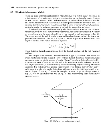
as a simple example the unidirectional flow of heat through a wall, as depicted in Fig. 27.
The temperature of the wall is not in general uniform but depends on both the time t and
position within the wall x, that is, (x, t). A distributed-parameter model for this case
might be the first-order partial differential equation
(x, t)
(x, t)
d 1 1
dt C xR x
t
t
where C is the thermal capacitance and R is the thermal resistance of the wall (assumed
t
t
uniform).
The complexity of distributed-parameter models is typically such that these models are
avoided in the analysis and design of control systems. Instead, distributed-parameter systems
are approximated by a finite number of spatial ‘‘lumps,’’ each lump being characterized by
some average value of the state. By eliminating the independent spatial variables, the result
is a lumped-parameter (or lumped-element) model described by coupled ordinary differential
equations. If a sufficiently fine-grained representation of the lumped microstructure can be
achieved, a lumped model can be derived that will approximate the distributed model to any
desired degree of accuracy. Consider, for example, the three temperature lumps shown in
Fig. 28, used to approximate the wall of Fig. 27. The corresponding third-order lumped
approximation is

Figure 27 Uniform heat transfer through a wall.