Page 377 - Mechanical Engineers' Handbook (Volume 2)

368 Mathematical Models of Dynamic Physical Systems 1 ƒ 1

ƒ
ƒ
i

x
x
x
n
2
1
ƒ
ƒ
ƒ
2
2
2

x
x
x
A(t) 1 2 n
ƒ
x
x n 1 ƒ n 2 ƒ n n
x
0
x(t) x 0 (t); u(t) u (t)

ƒ
ƒ
ƒ
1
1
1

u
u
u
m
1
2
ƒ
ƒ
ƒ
2
2
2

B(t) u 1 u 2 u m

ƒ
ƒ
n
n
ƒ n
u 1 u 2 u m
x(t) x 0 (t); u(t) u (t)
0
If the reference trajectory is a fixed operating point x, then the resulting linearized system
is time invariant and can be solved analytically. If the reference trajectory is a function of
time, however, then the resulting system is linear but time varying.
Describing Functions
The describing function method is an extension of the frequency transfer function approach
of linear systems, most often used to determine the stability of limit cycles of systems
containing nonlinearities. The approach is approximate and its usefulness depends on two
major assumptions:
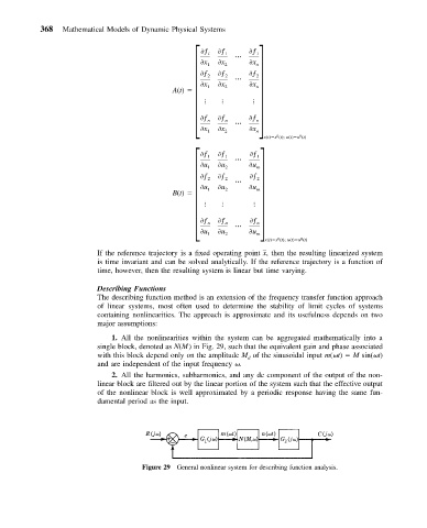
1. All the nonlinearities within the system can be aggregated mathematically into a
single block, denoted as N(M) in Fig. 29, such that the equivalent gain and phase associated
with this block depend only on the amplitude M of the sinusoidal input m( t) M sin( t)
d
and are independent of the input frequency .
2. All the harmonics, subharmonics, and any dc component of the output of the non-
linear block are filtered out by the linear portion of the system such that the effective output
of the nonlinear block is well approximated by a periodic response having the same fun-
damental period as the input.
Figure 29 General nonlinear system for describing function analysis.