Page 366 - Mechanical Engineers' Handbook (Volume 2)

7 Simulation 357
ƒ (k) b ƒ[˜x(k j), u(k j)]
N
˜
i
j 0 j i
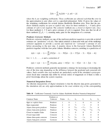
where the b are weighting coefficients. These coefficients are selected such that the error in
j
the approximation is zero when x (t) is a specified polynomial. Table 10 gives the values of
i
the weighting coefficients for several Adams–Bashforth–Moulton rules. Note that the pre-
dictor methods employ an open or explicit rule, since for these methods b 0 and a prior
0
estimate of x (k) is not required. The corrector methods use a closed or implicit rule, since
i
for these methods b
0 and a prior estimate of x (k) is required. Note also that for all of
i
i
these methods N j 0 b 1, ensuring unity gain for the integration of a constant.
j
Predictor–Corrector Methods
Predictor–corrector methods use one of the multistep predictor equations to provide an initial
estimate (or ‘‘prediction’’) of x(k). This initial estimate is then used with one of the multistep
corrector equations to provide a second and improved (or ‘‘corrected’’) estimate of x(k)
before proceeding to the next step. A popular choice is the four-point Adams–Bashforth
predictor together with the four-point Adams–Moulton corrector, resulting in a prediction of
t
˜
˜
˜
˜
˜ x (k) ˜x (k 1) [55ƒ (k 1) 59ƒ (k 2) 37ƒ (k 3) 9ƒ (k 4)]
i i i i i i
24
for i 1, 2,..., n and a correction of
t
˜
˜
˜
˜ x (k) ˜x (k 1) {9ƒ [˜x(k), u(k)] 19ƒ (k 1) 5ƒ (k 2) ƒ (k 3)}
i
i
i
i
i
i
24
Predictor–corrector methods generally incorporate a strategy for increasing or decreasing the
size of the time step depending on the difference between the predicted and corrected x(k)
values. Such variable time step methods are particularly useful if the simulated system pos-
sesses local time constants that differ by several orders of magnitude or if there is little a
priori knowledge about the system response.
Numerical Integration Errors
An inherent characteristic of digital simulation is that the discrete data points generated by
the simulation x(k) are only approximations to the exact solution x(t ) at the corresponding
k
Table 10 Coefficients Commonly Used for Adams–Bashforth–Moulton Numerical Integration 6
Predictor or
Common Name Corrector Points b 1 b 0 b 1 b 2 b 3
Open or explicit Euler Predictor 1 0 1 0 0 0
1
Open trapezoidal Predictor 2 0 3 ⁄2 ⁄2 0 0
16
Adams three-point predictor Predictor 3 0 23 ⁄12 ⁄12 5 ⁄12 0
59
9
Adams four-point predictor Predictor 4 0 55 ⁄24 ⁄24 37 ⁄24 ⁄24
Closed or implicit Euler Corrector 1 1 0 0 0 0
Closed trapezoidal Corrector 2 1 ⁄2 1 ⁄2 0 0 0
1
Adams three-point corrector Corrector 3 5 ⁄12 8 ⁄12 ⁄12 0 0
5
Adams four-point corrector Corrector 4 9 ⁄24 19 ⁄24 ⁄24 1 ⁄24 0