Page 40 - Mechanical Engineers' Handbook (Volume 2)

3 Statistics in the Measurement Process 29

ˆ 2 525
P[F F exp F ] F exp 1 1.33
R
L
ˆ 2 2 396
F F 0.05 ( , ) F 0.05 (14,10) 2.8
1
R
2
1 1
F F 0.95 ( , ) 0.385
L
2
1
F 0.05 (10,14) 2.60
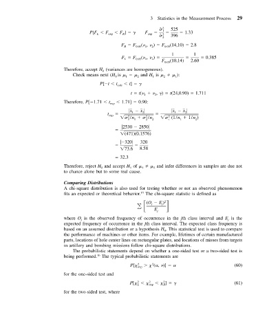
Therefore, accept H (variances are homogeneous).
0
Check means next (H is and H is
):
1
0
2
1
1
2
P[ t t calc t]
t t( , ) t(24,0.90) 1.711
2
1
Therefore, P[ 1.71 t exp 1.71] 0.90:
x x x x
t exp 1 2 1 2
2
2
2
/n /n 2 (1/n 1/n )
1
c
1
1
2
2
2530 2850

(471)(0.1576)
320 320

73.6 8.58
32.3
and accept H of
and infer differences in samples are due not
Therefore, reject H 0 1 1 2
to chance alone but to some real cause.
Comparing Distributions
A chi-square distribution is also used for testing whether or not an observed phenomenon
15
fits an expected or theoretical behavior. The chi-square statistic is defined as
(O E ) 2
j
j
E
j
where O is the observed frequency of occurrence in the jth class interval and E is the
j
j
expected frequency of occurrence in the jth class interval. The expected class frequency is
based on an assumed distribution or a hypothesis H . This statistical test is used to compare
0
the performance of machines or other items. For example, lifetimes of certain manufactured
parts, locations of hole center lines on rectangular plates, and locations of misses from targets
in artillery and bombing missions follow chi-square distributions.
The probabilistic statements depend on whether a one-sided test or a two-sided test is
16
being performed. The typical probabilistic statements are
P[ 2 exp ( , )] (60)
2
for the one-sided test and
P[ 2 exp ] (61)
2
2
L
R
for the two-sided test, where