Page 35 - Mechanical Engineers' Handbook (Volume 2)

24 Instrument Statics

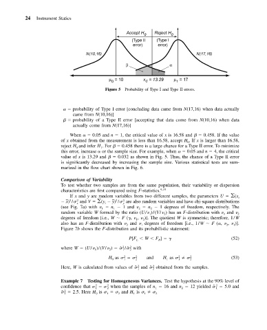
Figure 5 Probability of Type I and Type II errors.

probability of Type I error [concluding data came from N(17,16) when data actually
came from N(10,16)]

probability of a Type II error [accepting that data come from N(10,16) when data
actually come from N(17,16)]

When 0.05 and n 1, the critical value of x is 16.58 and
0.458. If the value
of x obtained from the measurement is less than 16.58, accept H .If x is larger than 16.58,
0
reject H and infer H .For
0.458 there is a large chance for a Type II error. To minimize
0 1
this error, increase or the sample size. For example, when 0.05 and n 4, the critical
value of x is 13.29 and
0.032 as shown in Fig. 5. Thus, the chance of a Type II error
is significantly decreased by increasing the sample size. Various statistical tests are sum-
marized in the flow chart shown in Fig. 6.

Comparison of Variability
To test whether two samples are from the same population, their variability or dispersion
characteristics are first compared using F-statistics. 9,15
If x and y are random variables from two different samples, the parameters U (x i
2
2
x)/ 2 x and V (y y)/ 2 y are also random variables and have chi-square distributions
i
(see Fig. 7a) with n 1 and n 1 degrees of freedom, respectively. The
2
2
1
1
random variable W formed by the ratio (U/ )/(V/ ) has an F-distribution with and 2
2
1
1
degrees of freedom [i.e., W
F ( , , )]. The quotient W is symmetric; therefore, 1/W
1
2
also has an F-distribution with and degrees of freedom [i.e., 1/W
F ( , , )].
2
1
2
1
Figure 7b shows the F-distribution and its probabilistic statement:
P[F W F ] (52)
L
R
where W (U/ )/(V/ ) ˆ /ˆ 2 with
2
1 2 1 2
2
2
H as 2 2 and H as
2 2 (53)
1
1
0
1
Here, W is calculated from values of ˆ 2 1 and ˆ 2 2 obtained from the samples.
Example 7 Testing for Homogeneous Variances. Test the hypothesis at the 90% level of
confidence that 2 2 when the samples of n 16 and n 12 yielded ˆ 2 1 5.0 and
2
1
2
1
ˆ 2 2 2.5. Here H is and H is
2
1
0
2
1
1