Page 415 - Mechanical Engineers' Handbook (Volume 2)

406 Basic Control Systems Design

G(s)H(s) 1, and the feedback elements must be selected so that H(s) 1/T(s). This
principle was used in Section 1 to explain the design of a feedback amplifier.

6.2 Electronic Controllers
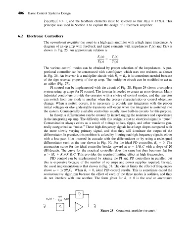
The operational amplifier (op amp) is a high-gain amplifier with a high input impedance. A
diagram of an op amp with feedback and input elements with impedances T (s) and T (s)is
ƒ i
shown in Fig. 25. An approximate relation is
E (s) T (s)
o ƒ
E (s) T (s)
i
i
The various control modes can be obtained by proper selection of the impedances. A pro-
portional controller can be constructed with a multiplier, which uses two resistors, as shown
in Fig. 26. An inverter is a multiplier circuit with R R . It is sometimes needed because
ƒ
i
of the sign reversal property of the op amp. The multiplier circuit can be modified to act as
an adder (Fig. 27).
PI control can be implemented with the circuit of Fig. 28. Figure 29 shows a complete
system using op amps for PI control. The inverter is needed to create an error detector. Many
industrial controllers provide the operator with a choice of control modes, and the operator
can switch from one mode to another when the process characteristics or control objectives
change. When a switch occurs, it is necessary to provide any integrators with the proper
initial voltages or else undesirable transients will occur when the integrator is switched into
the system. Commercially available controllers usually have built-in circuits for this purpose.
In theory, a differentiator can be created by interchanging the resistance and capacitance
in the integrating op amp. The difficulty with this design is that no electrical signal is ‘‘pure.’’
Contamination always exists as a result of voltage spikes, ripple, and other transients gen-
erally categorized as ‘‘noise.’’ These high-frequency signals have large slopes compared with
the more slowly varying primary signal, and thus they will dominate the output of the
differentiator. In practice, this problem is solved by filtering out high-frequency signals, either
with a low-pass filter inserted in cascade with the differentiator or by using a redesigned
differentiator such as the one shown in Fig. 30. For the ideal PD controller, R 0. The
1
attenuation curve for the ideal controller breaks upward at 1/R C with a slope of 20
2
dB/decade. The curve for the practical controller does the same but then becomes flat for
(R R )/R R C. This provides the required limiting effect at high frequencies.
1
2
1
2
PID control can be implemented by joining the PI and PD controllers in parallel, but
this is expensive because of the number of op amps and power supplies required. Instead,
the usual implementation is that shown in Fig. 31. The circuit limits the effect of frequencies
above 1/
R C . When R 0, ideal PID control results. This is sometimes called the
1
1
1
noninteractive algorithm because the effect of each of the three modes is additive, and they
do not interfere with one another. The form given for R 0isthe real or interactive
1

Figure 25 Operational amplifier (op amp). 1