Page 730 - Mechanical Engineers' Handbook (Volume 2)

3 State-Variable Selection and Canonical Forms 721

Here, q(t) satisfies the definition of a state vector since it has the same dimension as x(t).
Equations (15) and (16) are the state-space equations in terms of q(t). The matrices within
brackets in these equations are the modified system and coupling matrices.
As for continuous-time systems, the state vector for a given linear, discrete-time system
is not unique. Any vector q(k) related to a valid state vector x(k) by a constant, nonsingular
matrix T is also a valid state vector:
q(k) Tx(k) (17)
The corresponding state-space equations are
1
q(k 1) [TF(k)T ]q(k) [TG(k)]u(k) k k 0 (18)
y(k) [C(k)T ]q(k) [D(k)]u(k) k k 0 (19)
1
Since the state vector of a system is not unique, the selection of state variables for a
given application is governed by considerations such as ease of measurement of state vari-
ables or simplification of the resulting state-space equations. If the independent energy stor-
age elements in the system of interest are readily identified, selection of state variables
directly related to energy storage in the system is appropriate. An nth-order system has n
independent energy storage elements that would enable the selection of n state variables.
Examples of energy storage elements are springs and masses in mechanical systems, capac-
itors and inductors in electrical systems, and capacitance and inertance elements in fluid
(hydraulic and pneumatic) systems.
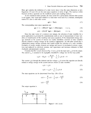
Consider the RLC circuit shown in Fig. 3. Let e (t) be the input and e (t) be the output.
in
out
The current i out is assumed to be negligible. Kirchhoff’s voltage law for the loop yields
di (t) 1
e (t) Ri (t) L in i (t) dt 0 (20)
in
in
in
dt C 1
The current i (t) through the inductor and the voltage e (t) across the capacitor are directly
out
in
related to energy storage in the system and are chosen as state variables:
x (t) i (t) (21)
1
in
1
x (t) e (t) i (t) dt (22)
2
in
out
C
1
The state equations can be determined from Eqs. (20)–(22) as
R 1 e (t)
˙ x (t) x (t) x (t) in (23)
2
1
1
L L L
x (t)
˙ x (t) 1 (24)
2
C 1
The output equation is

Figure 3 RLC circuit.