Page 729 - Mechanical Engineers' Handbook (Volume 2)

720 State-Space Methods for Dynamic Systems Analysis

where x, y, u state, output, and input vectors of the same dimensions as noted in con-
nection with Eqs. (1) and (2)
f, g same functions as in the equations already mentioned
t , t k 1 the kth and (k 1)th discrete-time instants, respectively
k
If the interval between consecutive discrete-time instants is constant and equal to T, and
if the functions f and g are linear, the state-space equations become
x(k 1) F(k)x(k) G(k)u(k) k k 0 (10)

y(k) C(k)x(k) D(k)u(k) k k 0 (11)
where the time instants kT and (k 1)T are represented by the corresponding sequence
numbers k and k 1, for notational convenience. In the preceding equations, F, G, C, and
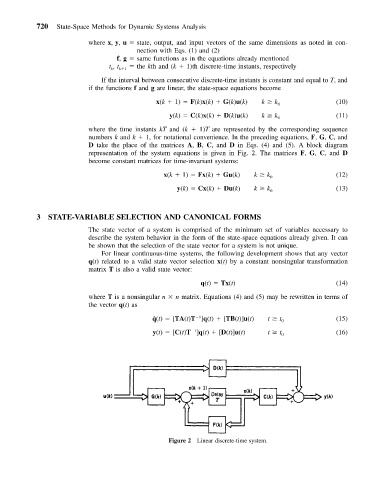
D take the place of the matrices A, B, C, and D in Eqs. (4) and (5). A block diagram
representation of the system equations is given in Fig. 2. The matrices F, G, C, and D
become constant matrices for time-invariant systems:
x(k 1) Fx(k) Gu(k) k k (12)
0
y(k) Cx(k) Du(k) k k (13)
0

3 STATE-VARIABLE SELECTION AND CANONICAL FORMS
The state vector of a system is comprised of the minimum set of variables necessary to
describe the system behavior in the form of the state-space equations already given. It can
be shown that the selection of the state vector for a system is not unique.
For linear continuous-time systems, the following development shows that any vector
q(t) related to a valid state vector selection x(t) by a constant nonsingular transformation
matrix T is also a valid state vector:

q(t) Tx(t) (14)
where T is a nonsingular n n matrix. Equations (4) and (5) may be rewritten in terms of
the vector q(t)as

1
˙ q(t) [TA(t)T ]q(t) [TB(t)]u(t) t t 0 (15)
y(t) [C(t)T ]q(t) [D(t)]u(t) t t 0 (16)
1

Figure 2 Linear discrete-time system.