Page 728 - Mechanical Engineers' Handbook (Volume 2)

2 State-Space Equations for Continuous-Time and Discrete-Time Systems 719

Equation (1) is the state equation and Eq. (2) is the output equation. The state, output, and
input vectors are

y (t)
x (t)
u (t)
1
1
1
u (t)
y (t)
x (t)
x(t) 2 y(t) 2 u(t) 2 (3)
x (t) y (t) u (t)
n
p
r
The elements x (t), x (t),..., x (t) of the state vector are the state variables of the system.
1
2
n
Formulation of the higher order system differential equations as a set of first-order
differential equations has the advantage that the latter are easier to solve by numerical meth-
ods than the former. If the functions f and g are linear functions of x(t) and u(t), the system
can be described by linear ordinary differential equations. Matrix notation can then be em-
ployed to simplify their representation:
˙ x(t) A(t)x(t) B(t)u(t) t t 0 (4)
y(t) C(t)x(t) D(t)u(t) t t 0 (5)
where A(t) n n system matrix
B(t) n r input–state coupling matrix
C(t) p n state–output coupling matrix
D(t) p r input–output transmission matrix
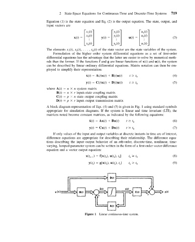
A block diagram representation of Eqs. (4) and (5) is given in Fig. 1 using standard symbols
appropriate for simulation diagrams. If the system is linear and time invariant (LTI), the
matrices noted become constant matrices, as indicated by the following equations:
˙ x(t) Ax(t) Bu(t) t t (6)
0
y(t) Cx(t) Du(t) t t (7)
0
If only values of the input and output variables at discrete instants in time are of interest,
difference equations are appropriate for describing their relationship. The difference equa-
tions describing the input–output behavior of an nth-order, discrete-time, nonlinear, time-
varying, lumped-parameter system can be written in the form of a first-order vector difference
equation and a vector output equation:
x(t k 1 ) f[x(t ), u(t ), t ] t t 0 (8)
k
k
k
k
y(t ) g[x(t ), u(t ), t ] t t 0 (9)
k
k
k
k
k

Figure 1 Linear continuous-time system.