Page 104 - Singiresu S. Rao-Mechanical Vibrations in SI Units, Global Edition-Pearson (2017)

1.11 harmoniC analysis 101
are known as half-range expansions [1.37]. Any of these half-range expansions can be
used to find x(t) in the interval 0 to t.

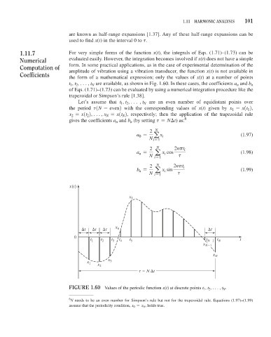
1.11.7 For very simple forms of the function x(t), the integrals of Eqs. (1.71)–(1.73) can be
numerical evaluated easily. However, the integration becomes involved if x(t) does not have a simple
Computation of form. In some practical applications, as in the case of experimental determination of the
amplitude of vibration using a vibration transducer, the function x(t) is not available in
Coefficients the form of a mathematical expression; only the values of x(t) at a number of points
t , t , c, t are available, as shown in Fig. 1.60. In these cases, the coefficients a and b
n
1 2
n
N
of Eqs. (1.71)–(1.73) can be evaluated by using a numerical integration procedure like the
trapezoidal or Simpson’s rule [1.38].
Let’s assume that t , t , c , t are an even number of equidistant points over
1 2
N
the period t1N = even2 with the corresponding values of x(t) given by x = x1t 2,
1
1
x = x1t 2, c, x = x1t 2, respectively; then the application of the trapezoidal rule
2
N
N
2
gives the coefficients a and b (by setting t = N t) as: 6
n
n
2 N
a = a i (1.97)
x
0
N i = 1
2 N 2npt i
x cos
a = a i (1.98)
n
N i = 1 t
2 N 2npt i
b = a i (1.99)
x sin
n
N i = 1 t
x(t)
x 5
t t t x 4 t
0
t 1 t 2 t 3 t 4 t 5 t N 1 t N t
x N 1
x N
x 1 x 2 x 3

t N t

FiGure 1.60 Values of the periodic function x(t) at discrete points t 1 , t 2 , c, t N .

6 N needs to be an even number for Simpson’s rule but not for the trapezoidal rule. Equations (1.97)–(1.99)
assume that the periodicity condition, x 0 = x N , holds true.