Page 403 - Mechanics of Asphalt Microstructure and Micromechanics

Characterization and Modeling Anisotropic Proper ties of Asphalt Concrete 395

P

θ X

r

Y z

ρ
σ z

τ rz

Z σ θ
σ
r
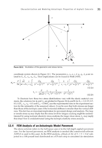
FIGURE 12.1 Illustration of the geometric and stress terms.

coordinate system shown in Figure 12.1. The parameters s 1 , s 2 , a, c, d, q 1 , q 2 , l, m are re-
lated to E v , E h , n vh , n hh , G vh . Their implications can be found in Wolf (1935).
⎧
P ⎪ d z ⎡ sq sq ⎤ λ z ⎡ sp sp
2
2
2
2
σ =− ⎨ − ⎢ 1 2 + 2 1 /2 ⎥ − 2 ⎢ 1 2 − 2 1
θ
−
22 3 2
22 3 2
2
2 223 2
2
22 3
⎩ ⎪
2 π ac d s 1 − s 2 ⎣ r ( 2 + s z ) / ( (r + s z ) ⎦ s − s r ⎣ (r + s z ) / (r 2 + s z ) /
2
2
2
1
1
1
(12-2a)
P z 1 1
τ =− [ − ]
22
2
rz π d s − s ( r + s z ) / ( r + s z )
2
22 3 2
2 1 2 1 2 (12-2b)
To illustrate how these two stress distributions vary with the elastic material con-
stants, the solutions for s θ and t yz are plotted in Figures 12.2a and b for E h = 1.0, 0.9, 0.7,
0.5, 0.2E v , n vh , n hh = 0.3 and G vh = 0.384E h (see the experimental data in the experiment sec-
tion for the rationality of the assumed values). It can be seen that both stresses are larger
than those of the isotropic cases if the horizontal stiffness is smaller than the vertical stiff-
ness. This fact has an important implication for pavement design and analysis. The larg-
er tensile stress s θ may imply that the stress level for fatigue cracking might be underes-
timated by using isotropic elasticity stress analysis; the larger shear stress t yz may imply
that shear flow is underestimated using the isotropic elasticity stress analysis.
12.4 FEM Analysis of an Anisotropic Model Pavement
The above solution refers to the half-space case or to the full-depth asphalt pavement
case. For the layered pavement, an FEM analysis is needed (the commercial software
3
ADINA is used in this case). In the FEM analysis, a block of AC of 5 5 3 in sub-
jected to a 100-pound load distributed on a 0.5-inch strip is simulated (in simulation