Page 406 - Mechanics of Asphalt Microstructure and Micromechanics

T
398 Ch a p t e r w e l v e

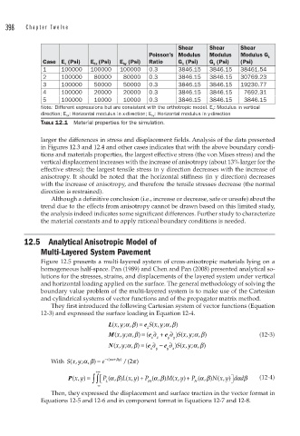
Shear Shear Shear
Poisson’s Modulus Modulus Modulus G z
Case E v (Psi) E hx (Psi) E hy (Psi) Ratio G x (Psi) G y (Psi) (Psi)
1 100000 100000 100000 0.3 3846.15 3846.15 38461.54
2 100000 80000 80000 0.3 3846.15 3846.15 30769.23
3 100000 50000 50000 0.3 3846.15 3846.15 19230.77
4 100000 20000 20000 0.3 3846.15 3846.15 7692.31
5 100000 10000 10000 0.3 3846.15 3846.15 3846.15
Note: Different expressions but are consistent with the orthotropic model. E v : Modulus in vertical
direction; E hx : Horizontal modulus in x-direction; E hy : Horizontal modulus in y-direction
TABLE 12.1 Material properties for the simulation.

larger the differences in stress and displacement fields. Analysis of the data presented
in Figures 12.3 and 12.4 and other cases indicates that with the above boundary condi-
tions and materials properties, the largest effective stress (the von Mises stress) and the
vertical displacement increases with the increase of anisotropy (about 13% larger for the
effective stress); the largest tensile stress in y direction decreases with the increase of
anisotropy. It should be noted that the horizontal stiffness (in y direction) decreases
with the increase of anisotropy, and therefore the tensile stresses decrease (the normal
direction is restrained).
Although a definitive conclusion (i.e., increase or decrease, safe or unsafe) about the
trend due to the effects from anisotropy cannot be drawn based on this limited study,
the analysis indeed indicates some significant differences. Further study to characterize
the material constants and to apply rational boundary conditions is needed.

12.5 Analytical Anisotropic Model of
Multi-Layered System Pavement
Figure 12.5 presents a multi-layered system of cross-anisotropic materials lying on a
homogeneous half-space. Pan (1989) and Chen and Pan (2008) presented analytical so-
lutions for the stresses, strains, and displacements of the layered system under vertical
and horizontal loading applied on the surface. The general methodology of solving the
boundary value problem of the multi-layered system is to make use of the Cartesian
and cylindrical systems of vector functions and of the propagator matrix method.
They first introduced the following Cartesian system of vector functions (Equation
12-3) and expressed the surface loading in Equation 12-4.
L(, ; , )xy αβ = e (, ; , )S xy αβ
z
M(, ; , ) (xy αβ = e ∂ + e ∂ Sx y)( , ; , )αβ (12-3)
x x y y y
N (, αβ ∂ − e ∂ ) S xy; ,β)
β
α
xy; , ) (e=
(,
x y y x
+
With Sx y; , )αβ = e − i(α x β y) /( π )
2
(,
+∞
αβ
αβ
xy ⎤
+
+
αβ
P(, )xy = ⎣ ∫ ∫ ⎡ P L ( , ) (, ) P M ( , ) (, ) P N ( , )N((, ) d dαβ (12-4)
L
⎦
M
xy
xy
−∞
Then, they expressed the displacement and surface traction in the vector format in
Equations 12-5 and 12-6 and in component format in Equations 12-7 and 12-8.