Page 423 - Mechanics of Asphalt Microstructure and Micromechanics

Characterization and Modeling Anisotropic Proper ties of Asphalt Concrete 415

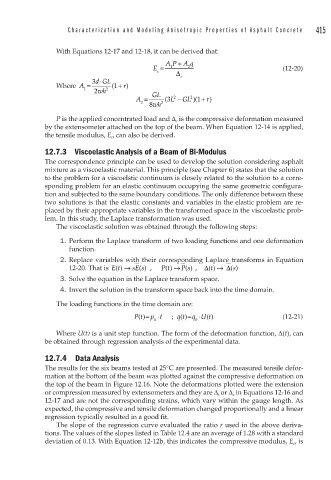
With Equations 12-17 and 12-18, it can be derived that:
+
AP A q
E = 1 2 (12-20)
c Δ
3 ⋅ c
Where A = dGL ( 1+ r)
1 2
2 wh
A = GL 3 ( L − GL 1+)( r)
2
2
2 8 wh 2
P is the applied concentrated load and Δ c is the compressive deformation measured
by the extensometer attached on the top of the beam. When Equation 12-14 is applied,
the tensile modulus, E t , can also be derived.
12.7.3 Viscoelastic Analysis of a Beam of Bi-Modulus
The correspondence principle can be used to develop the solution considering asphalt
mixture as a viscoelastic material. This principle (see Chapter 6) states that the solution
to the problem for a viscoelstic continuum is closely related to the solution to a corre-
sponding problem for an elastic continuum occupying the same geometric configura-
tion and subjected to the same boundary conditions. The only difference between these
two solutions is that the elastic constants and variables in the elastic problem are re-
placed by their appropriate variables in the transformed space in the viscoelastic prob-
lem. In this study, the Laplace transformation was used.
The viscoelastic solution was obtained through the following steps:

1. Perform the Laplace transform of two loading functions and one deformation
function.
2. Replace variables with their corresponding Laplace transforms in Equation
12-20. That is Et() → sE s) , Pt() → P s) , Δ t () → Δ s ( )
(
(
3. Solve the equation in the Laplace transform space.
4. Invert the solution in the transform space back into the time domain.

The loading functions in the time domain are:
⋅
⋅
Pt()= p t ; qt()= q U t() (12-21)
0 0
Where U(t) is a unit step function. The form of the deformation function, Δ(t), can
be obtained through regression analysis of the experimental data.
12.7.4 Data Analysis
The results for the six beams tested at 25°C are presented. The measured tensile defor-
mation at the bottom of the beam was plotted against the compressive deformation on
the top of the beam in Figure 12.16. Note the deformations plotted were the extension
or compression measured by extensometers and they are Δ t or Δ c in Equations 12-16 and
12-17 and are not the corresponding strains, which vary within the gauge length. As
expected, the compressive and tensile deformation changed proportionally and a linear
regression typically resulted in a good fit.
The slope of the regression curve evaluated the ratio r used in the above deriva-
tions. The values of the slopes listed in Table 12.4 are an average of 1.28 with a standard
deviation of 0.13. With Equation 12-12b, this indicates the compressive modulus, E c , is