Page 93 - Mechanics of Asphalt Microstructure and Micromechanics

86 Ch a p t e r Th r e e

binder may have a larger concentration of micro-pores and therefore become weak. In
addition, the spacing between two cavities, cracks, or solid inclusions is a measure of
their interaction. The mean spacing and the spacing variation may serve as good mea-
surements of how the weakening effects of two cavities can be magnified. This section
presents methods to quantify a set of damage parameters including the specific dam-
aged surface area tensor, the damage tensor, the average size of the cracks, the mean
solid path among the damaged surfaces, and the mean solid path tensor. This section
also presents the relationship between the quantified damage parameters and their ap-
plications in mechanical modeling. This work is applied, in particular, to quantify
damage parameters of AC specimens of the WesTrack project.
3.5.1 Fabric Tensor and Stereology Method
Unlike the cases for contact normal, branch vector, and orientation tensor, which are
actually inaccessible parameters, parameters in this section are accessible and can be
evaluated using statistics within the framework of stereology. Kanatani (1984a, 1984b,
1985) presented a systematic approach using the Buffon transform and fabric tensors to
represent the orientational distribution of geometric quantities. In these papers, Kana-
tani used a generic term “fabric” to represent the orientational distribution or arrange-
ment of any geometric and/or microstructural quantities. This approach, in conjunc-
tion with automated image analysis, can be used to determine the damage parameters
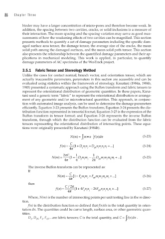
efficiently. Equation 3-23 presents the Buffon transform; Equation 3-24 presents the dis-
tribution function represented in tensorial format; Equation 3-25 is the expression of the
Buffon transform in tensor format; and Equation 3-26 represents the inverse Buffon
transform, through which the distribution function can be evaluated from the fabric
tensors representing the orientational distribution of intersecting points. These equa-
tions were originally presented by Kanatani (1984b).
•
Nm() = ∫ m n f n dn (3-23)
(
)
C
fn) = [ + Dn n + D n n n n + ...] (3-24)
(
1
4π ij i j ijkl i j k l
2π C 1 1
Nm) = [ + Dm m − D m m m m + ...] ] (3-25)
(
1
4π 4 ij i j 24 ijkl i j k l
The inverse Buffon transform can be represented as:
If
C
Nm) = [ + Fm m + F m m m m + ...] (3-26)
1
(
4π ij i j ijkl i j k l
then C/2π
fn() = [ + Fn n − 24 F n n n n + ...] (3-27)
14
4π ij i j ijkl i j k l
Where, N(m) is the number of intersecting points per unit testing line in the m direc-
tion.
f(n) is the distribution function so defined that f(n)dn is the total quantity in orien-
tation dn. The quantities could be curve length, surface area, or other geometric quan-
tities.
∫
D ij , D ijkl, F ij , F ijkl …are fabric tensors; C is the total quantity, and C = f(n)dn .