Page 34 - Mechanics of Microelectromechanical Systems

1. Stiffness basics 21
Two reaction forces correspond to the simply-supported boundary
condition of Fig 1.14 (c), whereas the fixed end of Fig. 1.14 (d) adds a
reaction moment to the forces of the previous case. It should be noted that for
a line member, three equilibrium equations can be written, and therefore the
boundary conditions should introduce three unknown reactions only, in order
for the system to be statically determinate. When less than three reactions are
present, the respective system is statically unstable (it is actually a
mechanism). For more than three unknown reactions, the system is statically
indeterminate, and additional equations need to be added to the equilibrium
ones, in order to determine the reaction loads.

5. LOAD-DISPLACEMENT CALCULATION
METHODS: CASTIGLIANO’S THEOREMS

5.1 Castigliano’s Theorems

There are several methods that can be utilized to determine the
deformations in an elastic body. In the case of bending for instance,
procedures exist to find the slope and deflection, such as the direct
integration method of the differential equation of beam flexure – Eq. (1.53),
the area-moment method or the Myosotis method. More generic methods that
allow calculation of elastic deformations for any type of load are the energy
methods (such as the principle of virtual work or Castigliano’s theorems), the
variational methods (the methods of Euler, Rayleigh-Ritz, Galerkin or
Trefftz), and the finite element method. Castigliano’s methods are
particularly useful when attempting to determine the stiffness of various
elastic members, and they will be utilized in this work quite extensively.
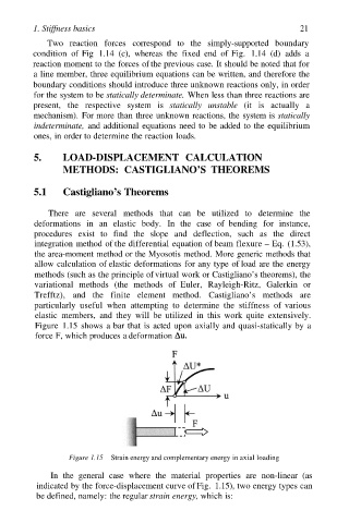
Figure 1.15 shows a bar that is acted upon axially and quasi-statically by a
force F, which produces a deformation

Figure 1.15 Strain energy and complementary energy in axial loading

In the general case where the material properties are non-linear (as
indicated by the force-displacement curve of Fig. 1.15), two energy types can
be defined, namely: the regular strain energy, which is: