Page 32 - Mechatronic Systems Modelling and Simulation with HDLs

2.4 MODEL DEVELOPMENT 21

the trivial conversion of a table model is the abrupt changes or kinks that are
caused by the fact that only a finite number of values are available. The difficulties
are numerical in nature since numerical oscillations may occur at abrupt changes
and kinks. These are caused by the fact that — as a result of feedback — different
sections of the characteristic are approached alternately and this may impair or
even prevent the convergence of the simulation. A possible solution is offered
by procedures that smooth the characteristic, such as the Chebychev or Spline
approximations.

Parameter estimation and system identification

In this connection we can differentiate between two aspects: Parameter estimation
and system identification. Parameter estimation requires a model and considers the
parameters that belong to it. Some parameters, such as mass or spring constants
are generally accessible without parameter estimation, whereas other parameters,
e.g. coefficients of friction, can often only be determined within the framework
of parameter estimation. The identified parameters then ensure the best possible
correspondence between simulation and measurement.
In system identification, on the other hand, a model for the system is created
on this basis or selected from a group of candidates. This is generally efficient
and numerically unproblematic. The quality criterion here is the degree of corre-
spondence that can be achieved using parameter estimation. The two significant
disadvantages of parameter estimation and system identification are that, firstly, a
measured result must be available in advance, which means that the system can
only be considered after its development and manufacture. Secondly, the results
are often not transferable, or at least not in a straightforward manner, to variations
of the system or of components.
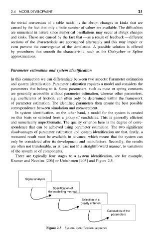
There are typically four stages to a system identification, see for example,
Kramer and Neculau [206] or Unbehauen [405] and Figure 2.5.

Signal analysis

Specification of
the modelling method

Selection of a
quality criterion
Calculation of the
parameters

Figure 2.5 System identification sequence