Page 34 - Mechatronic Systems Modelling and Simulation with HDLs

2.4 MODEL DEVELOPMENT 23

n k
x k Real
system y
a·x k k
e k
Q min
−
Model y ˆ k
â·x k â

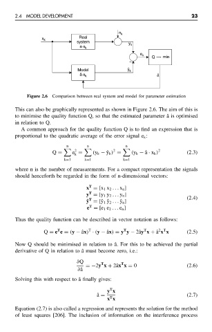
Figure 2.6 Comparison between real system and model for parameter estimation

This can also be graphically represented as shown in Figure 2.6. The aim of this is
to minimise the quality function Q, so that the estimated parameter ˆ a is optimised
in relation to Q.
A common approach for the quality function Q is to find an expression that is
proportional to the quadratic average of the error signal e k :

n n n

2 2 2
Q = e = (y k − ˆy k ) = (y k − ˆa · x k ) (2.3)
k
k=1 k=1 k=1
where n is the number of measurements. For a compact representation the signals
should henceforth be regarded in the form of n-dimensional vectors:

T
x = [x 1 x 2 ... x n ]
T
y = [y 1 y 2 ... y n ]
T
ˆ y = [ˆy 1 ˆy 2 ... ˆy n ] (2.4)
T
e = [e 1 e 2 ... e n ]
Thus the quality function can be described in vector notation as follows:
T
2 T
T
T
T
Q = e e = (y − ˆax) · (y − ˆax) = y y − 2ˆay x + ˆa x x (2.5)
Now Q should be minimised in relation to ˆ a. For this to be achieved the partial
derivative of Q in relation to ˆ a must become zero, i.e.:
∂Q T T
=−2y x + 2ˆax x = 0 (2.6)
∂ˆa
Solving this with respect to ˆ a finally gives:

T
y x
ˆ a = (2.7)
T
x x
Equation (2.7) is also called a regression and represents the solution for the method
of least squares [206]. The inclusion of information on the interference process