Page 100 - Mechatronics for Safety, Security and Dependability in a New Era

Ch18-I044963.fm Page 84 Tuesday, August 1, 2006 2:59 PM
Ch18-I044963.fm
84 84 Page 84 Tuesday, August 1, 2006 2:59 PM

u5x
0.3 0.3 - / • ; ; " : •"•• /"'. : \ " " • • - ' S l y • - - • • • -
._. ------ -- - u&x- ——— - J
u10x - 2 _„-,' , •' - 1 u10 y .
0.2 °- i 1 ' - i-f
j
0.1 men
0 - i u 0 - ' ;•_) r J ,-
-0.1 - <- i , , H -0.1
-0.2 ~° -0.2 -
-0.3 -0.3 -
-0.4 i i i i -0.4 1 1 1 1
time [s] time [s]
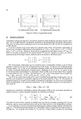
(a) displacements along .x-axis (b) displacements along j/-axis
Figure 3: Motion of positioned points
4 SIMULATION
Viscoelastie deformation has been extensively studied in solid mechanics and finite element anal-
ysis. Let us briefly describe the dynamic modeling of two-dimensional viscoelastie deformation.
Note that the deformation modeling is not for the control law of an ISP but for the simulation of
an ISP process.
Let o" be a pseudo stress vector and e be a psoudo strain vector. Stress-strain relationship of
vls
ela
2D isotropic viscoelastie deformation is formulated as a = (A/ A + /;/,,)£, where A = A + A d/d£
ela
ela
vls
and fi = /i + /x d/dt. Elasticity of the object is specified by two elastic moduli A and /i ela
vls
while its viscosity is specified by two viscous moduli A and //™. Matrices I\ and I fJ are matrix
representations of isotropic tensors, which arc given as follows in 2D deformation:
" 1 1 0 " • 2 0 0 "
1 1 0 . h = 0 2 0
0 0 0 0 0 1
The stress-strain relationship can be converted into a relationship between a set of forces
applied to nodal points and a set of displacements of the points. Let % be a set of displacements
of nodal points. Let J\ and J tl are connection matrices, which can be geometrically determined
by object coordinate components of nodal points. Replacing I\ by ,J\, 1^ by ,/,,, and e by tt K
in the stress-strain relationship of a viscoelastie object yields a set of viscoelastie forces applied
to nodal points as (\J\ + /iJ^u^. Introducing JI N = u N , a set of viscoelastie forces is given by
vis
+ Bv N, ela ela and B = A J A + ^™J M.
Ku N where K = A J A + /t J ;J
Let M be an inertia matrix and / be a set of external forces applied to nodal points. Let us
T
describe a set of geometric constraints imposed on the nodal points by .4 u^ = b. The number of
columns of matrix A is equal to the number of geometric constraints. Let A be a set of constraint
forces corresponding to the geometric constraints. A set of dynamic equations of nodal points is
then given by
M«N = —Kuy — Bvy + f + AX.
Applying the constraint stabilization method [Baumgarte 1972] to the constraints specified by
angular velocity to, system dynamic equations are described as follows:

M -A -Ku N - (3)
-,4 T -b)\
Note that the above linear equation is solvable since the matrix is regular, implying that we can
sketch uyt and D N using numerical solver such as the Euler method or the Runge-Kutta method.
Let us simulate an indirect simultaneous positioning by taking a simple example illustrated in
Figure 2. Two-dimensional deformation of a viscoelastie object is described by nodal points P o
through Pi, 5. Let us guide three points P l5, P 6 , and Pio to their desired location by controlling