Page 312 - Modeling of Chemical Kinetics and Reactor Design

282 Modeling of Chemical Kinetics and Reactor Design

F 3 ( )= K2* X 2 ( ) (5-72)

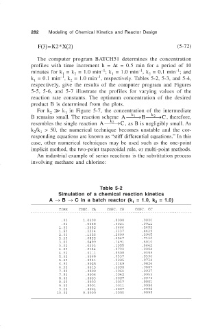
The computer program BATCH51 determines the concentration
profiles with time increment h = ∆t = 0.5 min for a period of 10
–1
–1
–1
minutes for k = k = 1.0 min ; k = 1.0 min , k = 0.1 min ; and
1
2
2
1
–1
–1
k = 0.1 min , k = 1.0 min , respectively. Tables 5-2, 5-3, and 5-4,
2
1
respectively, give the results of the computer program and Figures
5-5, 5-6, and 5-7 illustrate the profiles for varying values of the
reaction rate constants. The optimum concentration of the desired
product B is determined from the plots.
For k k k in Figure 5-7, the concentration of the intermediate
1
2
B remains small. The reaction scheme A → B  → , therefore,

k 1
k 2
C
resembles the single reaction A → C , as B is negligibly small. As
k 2
k /k > 50, the numerical technique becomes unstable and the cor-
2
1
responding equations are known as “stiff differential equations.” In this
case, other numerical techniques may be used such as the one-point
implicit method, the two-point trapezoidal rule, or multi-point methods.
An industrial example of series reactions is the substitution process
involving methane and chlorine:
Table 5-2
Simulation of a chemical reaction kinetics
A → B → C in a batch reactor (k = 1.0, k = 1.0)
1
2