Page 102 - Modern Analytical Chemistry

1400-CH04 9/8/99 3:54 PM Page 85

Chapter 4 Evaluating Analytical Data 85

The probability of a type 1 error is inversely related to the probability of a type
2 error. Minimizing a type 1 error by decreasing a, for example, increases the likeli-
hood of a type 2 error. The value of a chosen for a particular significance test,
therefore, represents a compromise between these two types of error. Most of the
examples in this text use a 95% confidence level, or a= 0.05, since this is the most
frequently used confidence level for the majority of analytical work. It is not
unusual, however, for more stringent (e.g. a = 0.01) or for more lenient
(e.g. a= 0.10) confidence levels to be used.

t exp s t exp s
4 F Statistical Methods for Normal Distributions X – n X + n

The most commonly encountered probability distribution is the normal, or Gauss-
ian, distribution. A normal distribution is characterized by a true mean, m, and vari- (a)
–
2
2
ance, s , which are estimated using X and s . Since the area between any two limits
of a normal distribution is well defined, the construction and evaluation of signifi-
cance tests are straightforward.
t exp s t exp s
X – X +
–
4 F.1 Comparing X to m n n
One approach for validating a new analytical method is to analyze a standard
sample containing a known amount of analyte, m. The method’s accuracy is judged (b)
–
by determining the average amount of analyte in several samples, X, and using X – t(a,n)s X + t(a,n)s
–
a significance test to compare it with m. The null hypothesis is that X and m are n n
the same and that any difference between the two values can be explained by in-
–
determinate errors affecting the determination of X. The alternative hypothesis is
–
that the difference between X and m is too large to be explained by indeterminate
error. t exp s t exp s
The equation for the test (experimental) statistic, t exp , is derived from the confi- X – n X + n
dence interval for m
t exp s
m=X ± 4.14
n
t(a,ns t(a,ns
)
)
Rearranging equation 4.14 X – X +
n n
m - X ´ n (c)
t exp = 4.15
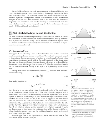
s Figure 4.11
Relationship between confidence intervals
gives the value of t exp when mis at either the right or left edge of the sample’s ap- and results of a significance test. (a) The
parent confidence interval (Figure 4.11a). The value of t exp is compared with a shaded area under the normal distribution
curves shows the apparent confidence
critical value, t(a,n), which is determined by the chosen significance level, a , the
intervals for the sample based on t exp . The
degrees of freedom for the sample, n, and whether the significance test is one- solid bars in (b) and (c) show the actual
tailed or two-tailed. Values for t(a,n) are found in Appendix 1B. The critical confidence intervals that can be explained by
indeterminate error using the critical value of
value t(a,n) defines the confidence interval that can be explained by indetermi-
(a,n). In part (b) the null hypothesis is
nate errors. If t exp is greater than t(a,n), then the confidence interval for the data rejected and the alternative hypothesis is
is wider than that expected from indeterminate errors (Figure 4.11b). In this case, accepted. In part (c) the null hypothesis is
retained.
the null hypothesis is rejected and the alternative hypothesis is accepted. If t exp is
less than or equal to t(a,n), then the confidence interval for the data could be at-
tributed to indeterminate error, and the null hypothesis is retained at the stated t-test
Statistical test for comparing two mean
significance level (Figure 4.11c). – values to see if their difference is too
A typical application of this significance test, which is known as a t-test of X to large to be explained by indeterminate
m, is outlined in the following example. error.