Page 112 - Modern Analytical Chemistry

1400-CH04 9/8/99 3:55 PM Page 95

Chapter 4 Evaluating Analytical Data 95

4 G Detection Limits

The focus of this chapter has been the evaluation of analytical data, including the
use of statistics. In this final section we consider how statistics may be used to char-
acterize a method’s ability to detect trace amounts of an analyte.
A method’s detection limit is the smallest amount or concentration of analyte detection limit
The smallest concentration or absolute
that can be detected with statistical confidence. The International Union of Pure
amount of analyte that can be reliably
and Applied Chemistry (IUPAC) defines the detection limit as the smallest concen- detected.
tration or absolute amount of analyte that has a signal significantly larger than the
signal arising from a reagent blank. Mathematically, the analyte’s signal at the detec-
tion limit, (S A ) DL , is
(S A ) DL = S reag + zs reag 4.25 Probability
distribution
where S reag is the signal for a reagent blank, s reag is the known standard devia- for blank
tion for the reagent blank’s signal, and z is a factor accounting for the desired
confidence level. The concentration, (C A ) DL , or absolute amount of analyte,
(n A ) DL , at the detection limit can be determined from the signal at the detection
limit. (a)
S reag (S )
A DL
)
(S ADL
(C ADL =
)
k
Probability distribution
for blank Probability
)
(S ADL distribution
(n ADL = for sample
)
k
The value for z depends on the desired significance level for reporting the detection
limit. Typically, z is set to 3, which, from Appendix 1A, corresponds to a signifi-
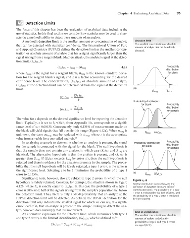
cance level of a= 0.00135. Consequently, only 0.135% of measurements made on
the blank will yield signals that fall outside this range (Figure 4.12a). When s reag is (b) S (S )
unknown, the term zs reag may be replaced with ts reag , where t is the appropriate reag A DL
value from a t-table for a one-tailed analysis. 13
In analyzing a sample to determine whether an analyte is present, the signal Probability distribution Probability
for the sample is compared with the signal for the blank. The null hypothesis is for blank distribution
for sample
that the sample does not contain any analyte, in which case (S A ) DL and S reag are
identical. The alternative hypothesis is that the analyte is present, and (S A ) DL is
greater than S reag . If (S A ) DL exceeds S reag by zs(or ts), then the null hypothesis is
rejected and there is evidence for the analyte’s presence in the sample. The proba-
bility that the null hypothesis will be falsely rejected, a type 1 error, is the same as
the significance level. Selecting z to be 3 minimizes the probability of a type 1
(c)
error to 0.135%. S reag (S )
A LOI
Significance tests, however, also are subject to type 2 errors in which the null
Figure 4.12
hypothesis is falsely retained. Consider, for example, the situation shown in Figure
Normal distribution curves showing the
4.12b, where S A is exactly equal to (S A ) DL. In this case the probability of a type 2 definition of detection limit and limit of
error is 50% since half of the signals arising from the sample’s population fall below identification (LOI). The probability of a type
1 error is indicated by the dark shading, and
the detection limit. Thus, there is only a 50:50 probability that an analyte at the
the probability of a type 2 error is indicated
IUPAC detection limit will be detected. As defined, the IUPAC definition for the by light shading.
detection limit only indicates the smallest signal for which we can say, at a signifi-
cance level of a, that an analyte is present in the sample. Failing to detect the ana-
lyte, however, does not imply that it is not present.
limit of identification
An alternative expression for the detection limit, which minimizes both type 1 The smallest concentration or absolute
and type 2 errors, is the limit of identification, (S A ) LOI , which is defined as 14 amount of analyte such that the
probability of type 1 and type 2 errors
(S A ) LOI = S reag + zs reag + zs samp are equal (LOI).