Page 113 - Modern Analytical Chemistry

1400-CH04 9/8/99 3:55 PM Page 96

96 Modern Analytical Chemistry

As shown in Figure 4.12c, the limit of identification is selected such that there is an
limit of quantitation
The smallest concentration or absolute equal probability of type 1 and type 2 errors. The American Chemical Society’s
amount of analyte that can be reliably Committee on Environmental Analytical Chemistry recommends the limit of
determined (LOQ). quantitation, (S A ) LOQ , which is defined as 15

S reag S A (S A ) LOQ = S reag +10s reag
Other approaches for defining the detection limit have also been developed. 16
The detection limit is often represented, particularly when used in debates over
public policy issues, as a distinct line separating analytes that can be detected from
17
those that cannot be detected. This use of a detection limit is incorrect. Defining
the detection limit in terms of statistical confidence levels implies that there may be
Never ??? Always
detected detected a gray area where the analyte is sometimes detected and sometimes not detected.
This is shown in Figure 4.13 where the upper and lower confidence limits are de-
Lower Upper
confidence confidence fined by the acceptable probabilities for type 1 and type 2 errors. Analytes produc-
interval interval ing signals greater than that defined by the upper confidence limit are always de-
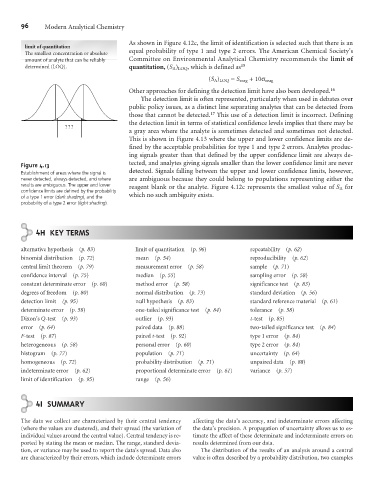
Figure 4.13 tected, and analytes giving signals smaller than the lower confidence limit are never
detected. Signals falling between the upper and lower confidence limits, however,
Establishment of areas where the signal is
never detected, always detected, and where are ambiguous because they could belong to populations representing either the
results are ambiguous. The upper and lower reagent blank or the analyte. Figure 4.12c represents the smallest value of S A for
confidence limits are defined by the probability
of a type 1 error (dark shading), and the which no such ambiguity exists.
probability of a type 2 error (light shading).

4 H KEY TERMS

alternative hypothesis (p. 83) limit of quantitation (p. 96) repeatability (p. 62)
binomial distribution (p. 72) mean (p. 54) reproducibility (p. 62)
central limit theorem (p. 79) measurement error (p. 58) sample (p. 71)
confidence interval (p. 75) median (p. 55) sampling error (p. 58)
constant determinate error (p. 60) method error (p. 58) significance test (p. 83)
degrees of freedom (p. 80) normal distribution (p. 73) standard deviation (p. 56)
detection limit (p. 95) null hypothesis (p. 83) standard reference material (p. 61)
determinate error (p. 58) one-tailed significance test (p. 84) tolerance (p. 58)
Dixon’s Q-test (p. 93) outlier (p. 93) t-test (p. 85)
error (p. 64) paired data (p. 88) two-tailed significance test (p. 84)
F-test (p. 87) paired t-test (p. 92) type 1 error (p. 84)
heterogeneous (p. 58) personal error (p. 60) type 2 error (p. 84)
histogram (p. 77) population (p. 71) uncertainty (p. 64)
homogeneous (p. 72) probability distribution (p. 71) unpaired data (p. 88)
indeterminate error (p. 62) proportional determinate error (p. 61) variance (p. 57)
limit of identification (p. 95) range (p. 56)

4I SUMMARY

The data we collect are characterized by their central tendency affecting the data’s accuracy, and indeterminate errors affecting
(where the values are clustered), and their spread (the variation of the data’s precision. A propagation of uncertainty allows us to es-
individual values around the central value). Central tendency is re- timate the affect of these determinate and indeterminate errors on
ported by stating the mean or median. The range, standard devia- results determined from our data.
tion, or variance may be used to report the data’s spread. Data also The distribution of the results of an analysis around a central
are characterized by their errors, which include determinate errors value is often described by a probability distribution, two examples