Page 126 - Modern Analytical Chemistry

1400-CH05 9/8/99 3:59 PM Page 109

Chapter 5 Calibrations, Standardizations, and Blank Corrections 109

analyte’s concentration. Thus, a multiple-point standardization should use at least
multiple-point standardization
three standards, although more are preferable. A plot of S stand versus C S is known as Any standardization using two or more
a calibration curve. The exact standardization, or calibration relationship, is deter- standards containing known amounts of
mined by an appropriate curve-fitting algorithm.* Several approaches to standard- analyte.
ization are discussed in the following sections.

5B.3 External Standards
The most commonly employed standardization method uses one or more external external standard
standards containing known concentrations of analyte. These standards are identi- A standard solution containing a known
fied as external standards because they are prepared and analyzed separately from amount of analyte, prepared separately
from samples containing the analyte.
the samples.
A quantitative determination using a single external standard was described at
the beginning of this section, with k given by equation 5.3. Once standardized, the
concentration of analyte, C A, is given as

S samp
C A = 5.4
k
5
EXAMPLE .2
A spectrophotometric method for the quantitative determination of Pb 2+ levels
in blood yields an S stand of 0.474 for a standard whose concentration of lead is
1.75 ppb. How many parts per billion of Pb 2+ occur in a sample of blood if
S samp is 0.361? S stand
SOLUTION
Equation 5.3 allows us to calculate the value of k for this method using the data
for the standard
.
S stand 0 474 –1 C A
k = = = 0 2709. ppb
.
C S 175 ppb (a)
Once k is known, the concentration of Pb 2+ in the sample of blood can be
calculated using equation 5.4
.
S samp 0 361
.
C A = = = 133 ppb
k 0 2709 ppb –1
.
S stand
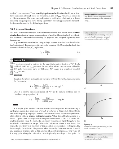
A multiple-point external standardization is accomplished by constructing a
calibration curve, two examples of which are shown in Figure 5.3. Since this is
the most frequently employed method of standardization, the resulting relation-
ship often is called a normal calibration curve. When the calibration curve is a
linear (Figure 5.3a), the slope of the line gives the value of k. This is the most de- C A
sirable situation since the method’s sensitivity remains constant throughout the (b)
standard’s concentration range. When the calibration curve is nonlinear, the
Figure 5.3
method’s sensitivity is a function of the analyte’s concentration. In Figure 5.3b,
Examples of (a) straight-line and (b) curved
for example, the value of k is greatest when the analyte’s concentration is small normal calibration curves.
and decreases continuously as the amount of analyte is increased. The value of
k at any point along the calibration curve is given by the slope at that point. In
normal calibration curve
A calibration curve prepared using
*Linear regression, also known as the method of least squares, is covered in Section 5C. several external standards.