Page 172 - Modern Control of DC-Based Power Systems

136 Modern Control of DC-Based Power Systems

The solution of the Eq. (5.72) allows the calculation of the final con-
trol law. The equation must guarantee that the trajectories of z converge
to z 5 0.

(5.72)
_ z 5 fzðÞ
If the application of the control law is able to drive to zero the off-
the-manifold trajectories and it guarantees that the trajectories of the
closed loop are bounded, then x is the asymptotically stable equilibrium

point of the closed-loop system. In calculation of the control law, the
Lyapunov function is not used, but the authors in [28] have demonstrated
that the mapping procedure represents the dual of the I&I approach.
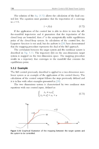
The correlation between the target system and the nonlinear system is
described in Fig. 5.13. The trajectory ξðtÞ on the one-dimension target
system is mapped on the two-dimension space. The mapping procedure
results in a trajectory that converges to the manifold that contains the
equilibrium point.

5.3.2 Example

The I&I control previously described is applied to a two-dimension non-
linear system as an example of the application of the control theory. The
calculation of the control output follows the steps previously defined and
it is in line with other examples presented in [28].
The two dimensions system is characterized by two nonlinear state
equations with one control input, defined as:
3
_ x 1 5 x 1 x 2
2
_ x 2 5 x 1 x 1 1 u (5.73)
2

x 2

π (ξ)
x (t)
M

0 ξ (t) ξ 1
x 1

Figure 5.13 Graphical illustration of the mapping between the target system and
the system to be controlled.