Page 56 - Modern Optical Engineering The Design of Optical Systems

Paraxial Optics and Calculations 39

These two equations are useful when the quantity of interest is the
distance l′. If the object and image are at the axial intersection distances
l and l′, the magnification is given by
h′ nl′
m (3.15b)
h n′l
In Sec. 2.2 we noted that the power of an optical system was the recip-
rocal of its effective focal length. In Eq. 3.15a the term (n′ n)/R is the
power of the surface. A surface with positive power will bend (converge)
a ray toward the axis; a negative-power surface will bend (diverge) a
ray away from the axis. If R is in meters, the power is in diopters.

3.3 Paraxial Raytracing through Several
Surfaces
The ynu raytrace
Another form of the paraxial equations is more convenient for use
when calculations are to be continued through more than one surface.
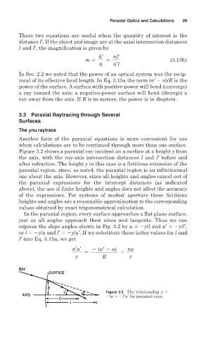
Figure 3.2 shows a paraxial ray incident on a surface at a height y from
the axis, with the ray-axis intersection distances l and l′ before and
after refraction. The height y in this case is a fictitious extension of the
paraxial region, since, as noted, the paraxial region is an infinitesimal
one about the axis. However, since all heights and angles cancel out of
the paraxial expressions for the intercept distances (as indicated
above), the use of finite heights and angles does not affect the accuracy
of the expressions. For systems of modest aperture these fictitious
heights and angles are a reasonable approximation to the corresponding
values obtained by exact trigonometrical calculation.
In the paraxial region, every surface approaches a flat plane surface,
just as all angles approach their sines and tangents. Thus we can
express the slope angles shown in Fig. 3.2 by u y/l and u′ y/l′,
or l y/u and l′ y/u′. If we substitute these latter values for l and
l′ into Eq. 3.15a, we get
n′u′ (n′ n) nu

y R y

Figure 3.2 The relationship y
lu l′u′ for paraxial rays.