Page 60 - Modern Optical Engineering The Design of Optical Systems

Paraxial Optics and Calculations 43

Note that the choice of y or u may be an arbitrary one. We can scale
1 1
y and u, but l and and l′ remain the same.
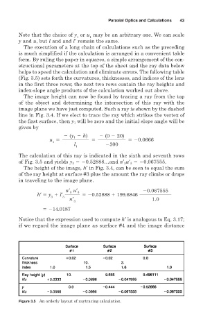
The execution of a long chain of calculations such as the preceding
is much simplified if the calculation is arranged in a convenient table
form. By ruling the paper in squares, a simple arrangement of the con-
structional parameters at the top of the sheet and the ray data below
helps to speed the calculation and eliminate errors. The following table
(Fig. 3.5) sets forth the curvatures, thicknesses, and indices of the lens
in the first three rows; the next two rows contain the ray heights and
index-slope angle products of the calculation worked out above.
The image height can now be found by tracing a ray from the top
of the object and determining the intersection of this ray with the
image plane we have just computed. Such a ray is shown by the dashed
line in Fig. 3.4. If we elect to trace the ray which strikes the vertex of
the first surface, then y 1 will be zero and the initial slope angle will be
given by
h) (0 20)
(y 1
u 0.0666
1
l 300
1
The calculation of this ray is indicated in the sixth and seventh rows
of Fig. 3.5 and yields y 3 0.52888…and n′ 3 u′ 3 0.067555.
The height of the image, h′ in Fig. 3.4, can be seen to equal the sum
of the ray height at surface #3 plus the amount the ray climbs or drops
in traveling to the image plane.
u′
n′ 3 3 0.067555
h′ y l′ 0.52888 199.6846
3 3
n′ 1.0
3
14.0187
Notice that the expression used to compute h′ is analogous to Eq. 3.17;
if we regard the image plane as surface #4 and the image distance

Figure 3.5 An orderly layout of raytracing calculation.