Page 57 - Modern Optical Engineering The Design of Optical Systems

40 Chapter Three

and multiplying through by y, we find the slope after refraction.
(n′ n)
n′u′ nu y (3.16)
R
It is frequently convenient to express the curvature of a surface as the
reciprocal of its radius, C 1/R; making this substitution, we have
n′u′ nu y (n′ n) C (3.16a)

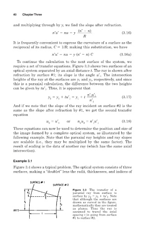
To continue the calculation to the next surface of the system, we
require a set of transfer equations. Figure 3.3 shows two surfaces of an
optical system separated by an axial distance t. The ray is shown after
refraction by surface #1; its slope is the angle u′ 1 . The intersection
heights of the ray at the surfaces are y 1 and y 2 , respectively, and since
this is a paraxial calculation, the difference between the two heights
can be given by tu′ 1 . Thus, it is apparent that
n′ 1u′ 1
y y tu′ y t (3.17)
2 1 1 1 n′
1
And if we note that the slope of the ray incident on surface #2 is the
same as the slope after refraction by #1, we get the second transfer
equation
u u′ or n u n′ u′ (3.18)
2 1 2 2 1 1
These equations can now be used to determine the position and size of
the image formed by a complete optical system, as illustrated by the
following example. Note that the paraxial ray heights and ray slopes
are scalable (i.e., they may be multiplied by the same factor). The
result of scaling is the data of another ray (which has the same axial
intersection).

Example 3.1
Figure 3.4 shows a typical problem. The optical system consists of three
surfaces, making a “doublet” lens the radii, thicknesses, and indices of

Figure 3.3 The transfer of a
paraxial ray from surface to
surface by y 2 y 1 tu′ 1 . Note
that although the surfaces are
drawn as curved in the figure,
mathematically they are treated
as planes. Thus the ray is
assumed to travel the axial
spacing t in going from surface
#1 to surface #2.