Page 62 - Modern Optical Engineering The Design of Optical Systems

Paraxial Optics and Calculations 45

ef l 122.950820
bf l 113.504098
ff l 124.590164

The ef l from the (right to left) calculation of ffl should be exactly the
same as the ef l from the (left to right) calculation for bfl.
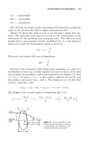
Figure 3.6 shows the path of such a ray through a single lens ele-
ment. The principal plane (p 2 ) is located by the intersection of the
extensions of the incident and emergent rays. The effective focal
length (ef l) or focal length (usually symbolized by f ), is the distance
from p 2 to f 2 and, for the paraxial region, is given by
y 1
ef l f
u′
2
The back focal length (bfl) can be found from

y 2
bf l
u′
2
Because of the frequency with which these quantities are used, it is
worthwhile to work up a single equation for each of them. If the lens
has an index of refraction n and is surrounded by air of index 1.0, then
n 1 n′ 2 1.0 and n′ 1 n 2 n. The surface radii are R 1 and R 2 , and
the surface curvatures are c 1 and c 2 . The thickness is t. At the first
surface, using Eq. 3.16a,
n′ u′ n u (n′ n ) y c 0 (n 1) y c
1 1 1 1 1 1 1 1 1 1
The height at the second surface is found from Eq. 3.17:
u′
tn′ 1 1 t (n 1) y c (n 1)
1 1
y y y y 1 tc
2 1 n′ 1 1 n 1
1 n

Figure 3.6 A ray parallel to the
axis is traced through an element
to determine the effective focal
length and back focal length.