Page 66 - Modern Optical Engineering The Design of Optical Systems

Paraxial Optics and Calculations 49

Noting that for an equiconvex lens R 1 R 2 , we use Eq. 3.25a to solve
for the radii
1 1 1 2

0.06 (n 1) 0.5
f R R R
1 2 1
1
R 16.67 mm
1
0.06
R R 16.67 mm
2 1

3.6 Mirrors
A curved mirror surface has a focal length and is capable of forming
images just as a lens does. The equations for paraxial raytracing
(Eqs. 2.31 and 2.32) can be applied to reflecting surfaces by taking into
account two additional sign conventions. The index of refraction of a
material was defined in the first chapter as the ratio of the velocity of
light in vacuum to that in the material. Since the direction of propa-
gation of light is reversed upon reflection, it is logical that the sign of
the velocity should be considered reversed, and the sign of the index
reversed as well. Thus the conventions are as follows:

1. The signs of the indices following a reflection are reversed, so the
index is negative when light travels right to left.
2. The signs of the spacings following a reflection are reversed if the
following surface is to the left.
Obviously if there are two reflecting surfaces in a system, the signs
of the indices and spacings are changed twice and, after the second
change, revert to the original positive signs, since the direction of propa-
gation is again left to right.
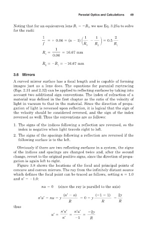
Figure 3.8 shows the locations of the focal and principal points of
concave and convex mirrors. The ray from the infinitely distant source
which defines the focal point can be traced as follows, setting n 1.0
and n′ 1.0:
nu 0 (since the ray is parallel to the axis)

(n′ n) ( 1 1) 2y
n′u′ nu y 0 y
R R R
thus
n′u′ n′u′ 2y
u′
n′ 1 R