Page 157 - Modern Spatiotemporal Geostatistics

138 Modern Spatiotemporal Geostatistics — Chapter 7

The BME equation (Eq. 7.10) is a concise, general, and in some sense
beautiful representation of the spatiotemporal mapping problem. In addition,
the solution of the BME equation can be accomplished efficiently with the cur-
rent computing technology (in many cases the computational time required is
only a fraction of that needed for space/time regression methods; e.g., Serre
et al., 1998). As we shall see later, the BME equation (Eq. 7.10) can be ex-
tended to include several estimation points p kj (j — 1,..., p) simultaneously
(multipoint mapping). BME Equations 7.6-7.10 are, of course, all mathemat-
ical consequences of the general form of Equation 5.35 (p. 120). But there are
a few aspects here that are not obvious to the unaided intuition. The BME
equations, e.g., include a mechanism that allows them to distinguish between
hard (more accurate) data and soft (less accurate) data, and then assign the
appropriate weight to them. Furthermore, it should be remembered that, at
this stage, the Lagrange multipliers /i a have known values which are deter-
mined from the solution of the system of Equations 5.10 and 5.11 (p. 107)
and incorporate general knowledge §. Equation 7.10 is, in general, a nonlinear
equation of the estimate Xk, and may have more than one solution that in-
cludes more than one local maximum. In this case, the estimate is equal to the
largest local maximum of the pdf. The verification of the condition in Equa-
tion 7.4 and the search for the largest local maximum can be accomplished by
analytical means or numerical procedures. In order to study such aspects in
more detail, as well as to obtain explicit analytical expressions and numerical
results for the BME estimators, we will focus mainly on Equations 7.6 and 7.7
in the following examples. Of course, the analysis can be extended to any other
^-operator, as well.

Statistics—Hard and soft data

The next example serves to illustrate the step-by-step implementation of the
BMEmode approach in light of statistical knowledge and hard/soft data.

EXAMPLE 7.2: Consider the simple but instructive case of three points p x,
p 2, and p k. It is assumed that the prior knowledge includes the mean and
the centered ordinary covariance. Also, assume that there is a hard datum
(measurement) at point p^ and a soft datum (interval) at point p%. Based on
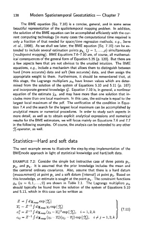
this knowledge, an estimate is sought at the point p k. The constraint functions
9a (of — 0,1,...,9) are shown in Table 7.1. The Lagrange multipliers [i a
should typically be found from the solution of the system of Equations 5.10
and 5.11, which in this case can be written as