Page 80 - Modern Spatiotemporal Geostatistics

Spatiotemporal Geometry 61

where g(-) is some known function. [Notice the difference between fir(x map),
which is a function of the realization values, and its expectation ~g(p map),
which is a function of the space/time points.] There is, generally, no need to
specify limits of integration in Equation 2.44, since if certain ranges of Xma P
are impossible, the pdf will be zero, removing contributions from these ranges.

EXAMPLE 2.27: If we let g(xi) = Xi< Equation 2.44 provides the mean

of the S/TRF. If we let g(xi,X2) = (Xi - zi)(X2 - x 2), the (centered)
covariance function

between the points p1 and p2 is obtained; etc.

COMMENT 2.11 : S/TRF characterization i n terms o f Equation 2.44 w

considered "incomplete" (or general or vague), in the sense that several
random fields exist that share the same space/time moments. Also, statisti-
cal moments can be defined for more than one random field simultaneously,

in which case Equation 2.44 should involve data or map vectors for all

these field s (see, e.g., th e multivariable o r vector formulation o f BM E i n

Chapter 9).

Correlation analysis and spatiotemporal geometry
In geostatistical applications, spatiotemporal correlation functions are usually
part of the available physical knowledge bases. These functions could be de-
rived from a physical law or fitted to the data. Commonly used correlation
functions include the ordinary covariance, the variogram (sometimes also called
semivariogram), and the generalized covariance. Ordinary covariance analysis,
e.g., can be helpful in determining the physically appropriate spatiotemporal
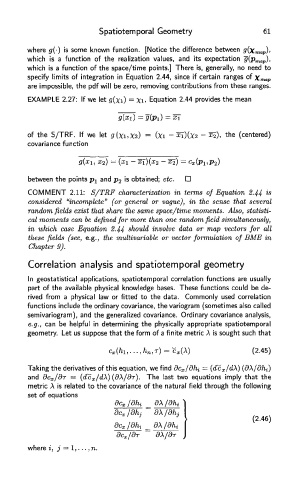
geometry. Let us suppose that the form of a finite metric A is sought such that

Taking the derivatives of this equation, we find dc x/dhi = (dc x/dX) (dX/dhi)
and dc x/dr = (dc x/dX) (dX/dr). The last two equations imply that the
metric A is related to the covariance of the natural field through the following
set of equations

where i, j = 1,... ,n.