Page 84 - Modern Spatiotemporal Geostatistics

Spatiotemporal Geometry 65

Proof: Since Equation 2.53 is a separable space/time function, we can study
spatial and temporal parts separately. We first concentrate on the spatial part

Let us suppose that c x(h) is a nonnegative definite function. Then, according
2
to Bochner's theorem, there exists a unique Borel measure fi x on R such that

Since c x (Aft) = exp[—A 2 \h\ } for all real A, the uniqueness of the Fourier
transform implies that k • h follows a one-dimensional Gaussian distribution
2
with variance 2 |ft| 2 = f R2 (k • ft.) d(j, x(k}. Hence, $ h(fc) = fc • ft. is square
integrable with respect to /x x, i.e., $/,(&) 6 Z/2(Mz)- The map ft. —> -4^ <5 h
2
becomes a norm preserving embedding (R , | • |) into L^^x)- It then follows
2
that (.R , | - | ) should be a Hilbert space—as a subspace of L<2(p, x). However,
2
if the norm | • | is defined as the distance (Eq. 2.54), (R , \ • \) is not a Hilbert
space, because we cannot define an inner product on R 2 such that |ft| =
(ft, ft-), which leads to a contradiction. Therefore, we conclude that c x(h) is
not a nonnegative definite function.
In fact, a stronger result can be proven, i.e., that under some general
assumptions, the metric in Equation 2.55 must necessarily be Euclidean (Chris-
takos and Papanicolaou, 2000). The validity of Proposition 2.1 may be illus-
trated by means of a numerical example.

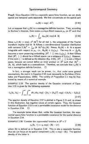
EXAMPLE 2.29: The spectral density of the Gaussian covariance of Equa-
tion 2.55 is given by the following expression

The spectral density of Equation 2.57 is plotted in Figure 2.15 and, as shown
in this illustration, has negative values at certain regions. Thus, the Gaussian
function of Equation 2.53 is not a permissible covariance model for the distance
in Equation 2.54.

The example below shows that, unlike the Gaussian function, the expo-
nential space/time function is a permissible covariance for the spatial distance
in Equation 2.54.
EXAMPLE 2.30: Consider the exponential function in R 2 x T

where \h\ is defined as in Equation 2.54. This is also a separable function,
thus we can focus on its spatial component c x(ft) = exp(- |ft.|). The spectral
density of the latter is