Page 82 - Modern Spatiotemporal Geostatistics

Spatiotemporal Geometry 63

A healthy dose of intuition and a deeper understanding of the physical
situation will also be of great value in determining 5^. Indeed, as we saw in a
previous section ("The Field Idea," p. 54), in light of the physical equations,
the spatiotemporal geometry and the natural variables are not independent of
one another; rather they are connected via these equations. As a result of
this connection, the behavior of the natural phenomenon is tied to space/time
itself. Consider the following example.
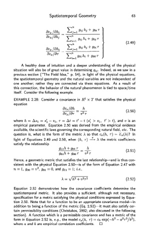
EXAMPLE 2.28: Consider a covariance in R 1 x T that satisfies the physical
equation

where h = Asj = s( — s\, T — At = t' - t (s( > si, t' > t), and v is an
empirical parameter. Equation 2.50 was derived from the empirical evidence
available, the scientific laws governing the corresponding natural field, etc. The
question is, what is the form of the metric A so that c x(h, r) = c x (A)? In
light of Equations 2.49 and 2.50, when (h, T) —> X the metric coefficients
satisfy the relationship

Hence, a geometric metric that satisfies the last relationship—and is thus con-
sistent with the physical Equation 2.50—is of the form of Equation 2.47 with
2
n = l, goo = v , g 0i = 0, and g n = 1; i.e.,

Equation 2.52 demonstrates how the covariance coefficients determine the
spatiotemporal metric. It also provides a sufficient, although not necessary,
specification for a metric satisfying the physical conditions expressed by Equa-
tion 2.50. Note that for a function to be an appropriate covariance model—in
addition to being a function of the metric (Eq. 2.52)—it must also satisfy cer-
tain permissibility conditions (Christakos, 1992; also discussed in the following
section). A function which is a permissible covariance and has a metric of the
2 2
2
2
form in Equation 2.52 is, e.g., the model c x(h, r) = GO exp(—/i — a r /6 ),
where a and b are empirical correlation coefficients.