Page 94 - Modern Spatiotemporal Geostatistics

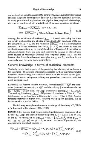
Physical Knowledge 75

and as closely as possible represent the general knowledge available from various
sciences. A specific formulation of Equation 3.1 deserves additional attention.
In many geostatistical applications, the physical laws, empirical relationships,
etc. can be transformed into a suitable set of moment equations as follows

s
where g a is a set of known functions of Xma P- '* ' worth mentioning that there
are certain mathematical and physical criteria involved in the choice of the g a.
By convention, go = 1, and the respective go(x map) = 1 is a normalization
constant. It is also necessary that the g a (a > 0) are chosen so that the
stochastic expectations h a on the left-hand side of Equation 3.2 can either be
calculated directly from field data and experimental surveys or inferred from
other sources of knowledge (physical laws, empirical charts, etc.}. As will
become clear from the subsequent examples, the g a and h a functions do not
necessarily have the same mathematical form.
General knowledge in terms of statistical moments

To clarify certain basic aspects of the preceding formulations, let us discuss a
few examples. The general knowledge considered in these examples includes
functions characterizing the statistical behavior of the natural system (spa-
tiotemporal means, variograms, ordinary and generalized covariances, multiple-
point statistics, etc.}.
2
EXAMPLE 3.3: Assume that the means x,, the variances (xi — a^) , the third-
3
order (centered) moments (xi - x^) , and the ordinary (centered) covariances
(xi — Xi) (xv — xF)of the S/TRF X(p) are known at pointsp it i = 1, ...,m,k.
The resulting functions g a(Xmap) °f Equation 3.2 are shown in Table 3.1. The
total number of g a functions in this case is 1 + (m + l)(m + 6)/2. Spatio-
temporal statistics of higher order, including multiple-point statistics, can be
incorporated in a similar fashion.

The following example requires some knowledge of the theory of S/TRF-
v/jj, developed in Christakos (1991b, 1992).
EXAMPLE 3.4: Assume that the generalized spatiotemporal covariances of an
S/TRF-1/1 X(p) are known between the points p i (i — 1,2,3,4, k). In view
2
of the S/TRF theory, we let g( Xrmp) = (Xk ~ lEti**) . where Xmap =
(Xi, X2, X.3, X4, Xk) and g Q = 1, as usual. In view of Equation 3.2, the
corresponding statistical function is