Page 98 - Modern Spatiotemporal Geostatistics

Physical Knowledge 79

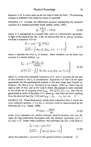
Equation 3.14, in many cases we do not need to solve for them. The preceding
analysis is exhibited most easily by means of examples.
EXAMPLE 3.7: Consider the differential equation representing the temporal
variation of a lumped parameter Earth system (Jones, 1997),

where X is represented as a random field, and b is a deterministic parameter.
In light of the physical law (Eq. 3.16), we assume that the h a and g a functions
involved in Equation 3.14 are

where a denotes the time t a of interest. Other statistics can be taken into
account in a similar fashion, e.g.,

where C x is the (non-centered) covariance of X, and a' accounts for the pair
of time instants tj and tj in consideration. Equations 3.17 and 3.18 are quite
appropriate for the geostatistical analysis in the prior stage (see Chapter 5).
However, the choice of g a/ functions is not unique. Other g a> forms may be
used as well. In fact, just as for Class A above, the analysis is easily extended
to the whole set of mapping times t map. The g a'(xi,Xj), e.g., may also be
generalized in terms of Equation 3.11, where g a> may have any form resulting
from the physical law (Eq. 3.16) and t map = (ti,... ,t m, *&); et
EXAMPLE 3.8: Three-dimensional, steady-state subsurface flow in which the
mean hydraulic gradient J is in the si direction could be approximated by the
following law (e.g., Dagan, 1989)

where X(s) represents the random hydraulic head fluctuation, and u(s) de-
notes the log-conductivity fluctuation with the isotropic covariance c u(r) =
CT^ exp[—r/e]. Under these conditions, the hydrologic law (Eq. 3.19) leads to

where the subscript a accounts for the spatial locations considered.