Page 96 - Modern Spatiotemporal Geostatistics

Physical Knowledge 77

procedure if it were carried out. The spatiotemporal distribution of most natural
variables is expressed through physical laws which, thus, constitute important
aspects of the mapping process. For the purposes of this book, two prime
classes of laws, A and B, will be considered.
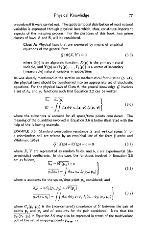
Class A: Physical laws that are expressed by means of empirical
equations of the general form

where $(•) is an algebraic function, X(p) is the primary natural
variable, and Y(p) = (Yi(p), . . . , ^it(p)) is a vector of secondary
(measurable) natural variables in space/time.

As was already mentioned in the section on mathematical formulation (p. 74),
the physical laws should be transformed into an appropriate set of stochastic
equations. For the physical laws of Class A, the general knowledge § involves
a set of h a and g a functions such that Equation 3.2 can be written

where the subscripts a account for all space/time points considered. The
meaning of the quantities involved in Equation 3.6 is better illustrated with the
help of the following example.

EXAMPLE 3.6: Standard penetration resistance X and vertical stress Y for
a cohesionless soil are related by an empirical law of the form (Lambe and
Whitman. 19691

where X, Y are represented as random fields, and -b, c are experimental (de-
terministic) coefficients. In this case, the functions involved in Equation 3.6
are as follows,

where a accounts for the space/time point p a considered; and

where C y(p i,pj) is the (non-centered) covariance of Y between the pair of
points p t and PJ and a' accounts for the pair considered. Note that the
y
9a'(xi, j) in Equation 3.9 may also be expressed in terms of the multivariate
pdf of the set of mapping points p map, i.e.,