Page 115 - Neural Network Modeling and Identification of Dynamical Systems

104 3. NEURAL NETWORK BLACK BOX APPROACH TO THE MODELING AND CONTROL OF DYNAMICAL SYSTEMS

The problem is to select the transformation
implemented by the controller so that this con-
trolled system would show the behavior closest
to the behavior of the reference model. This task
we call the task of adjusting the dynamic properties
of the plant.
The task of adjusting the dynamic properties
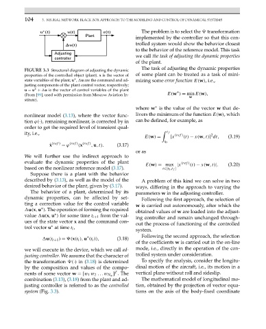
FIGURE 3.3 Structural diagram of adjusting the dynamic
properties of the controlled object (plant). x is the vector of of some plant can be treated as a task of mini-
∗
state variables of the plant; u , u are the command and ad- mizing some error function E(w), i.e.,
justing components of the plant control vector, respectively;
∗
u = u + u is the vector of control variables of the plant ∗
(From [99], used with permission from Moscow Aviation In- E(w ) = minE(w),
w
stitute).
where w is the value of the vector w that de-
∗
nonlinear model (3.13), where the vector func- livers the minimum of the function E(w),which
tion ϕ(·), remaining nonlinear, is corrected by in can be defined, for example, as
order to get the required level of transient qual-

ity, i.e., t f (ref ) 2
E(w) = [x (t) − x(w,t)] dt, (3.19)
t 0
(ref )
(ref )
(ref )
˙ x = ϕ (x ,u,t). (3.17)
or as
We will further use the indirect approach to
evaluate the dynamic properties of the plant (ref )
E(w) = max |x (t) − x(w,t)|. (3.20)
based on the nonlinear reference model (3.17). t∈[t 0 ,t f ]
Suppose there is a plant with the behavior
described by (3.13), as well as the model of the A problem of this kind we can solve in two
desired behavior of the plant, given by (3.17). ways, differing in the approach to varying the
The behavior of a plant, determined by its parameters w in the adjusting controller.
dynamic properties, can be affected by set- Following the first approach, the selection of
ting a correction value for the control variable
w is carried out autonomously, after which the
∗
u(x,u ). The operation of forming the required
obtained values of w are loaded into the adjust-
∗
value u(x,u ) for some time t i+1 from the val- ing controller and remain unchanged through-
ues of the state vector x and the command con-
out the process of functioning of the controlled
∗
trol vector u at time t i ,
system.
Following the second approach, the selection
∗
u(t i+1 ) = (x(t i ),u (t i )), (3.18)
of the coefficients w is carried out in the on-line
we will execute in the device, which we call ad- mode, i.e., directly in the operation of the con-
justing controller. We assume that the character of trolled system under consideration.
the transformation (·) in (3.18) is determined To specify the analysis, consider the longitu-
by the composition and values of the compo- dinal motion of the aircraft, i.e., its motion in a
T
] .The vertical plane without roll and sideslip.
nents of some vector w =[w 1 w 2 ...w N w
combination (3.13), (3.18) from the plant and ad- The mathematical model of longitudinal mo-
justing controller is referred to as the controlled tion, obtained by the projection of vector equa-
system (Fig. 3.3). tions on the axis of the body-fixed coordinate