Page 117 - Neural Network Modeling and Identification of Dynamical Systems

106 3. NEURAL NETWORK BLACK BOX APPROACH TO THE MODELING AND CONTROL OF DYNAMICAL SYSTEMS

model (3.17), which for the case of the system
(3.23) takes the form
(ref )
dV z Z (ref )
= − V x q ,
dt m (3.25)
dq (ref ) M y (ref )
= .
dt I y
The condition mentioned above for M y in
(3.23)alsoholds for(3.25).
The reference model (3.25) differs from the
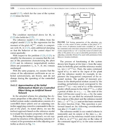
original model (3.23) by the expression for the FIGURE 3.4 Tuning parameters of the adjusting con-
(ref ) troller. x is the vector of state variables of the plant; x (ref )
moment of the pitch M y ,which,incompari- ∗
is the vector of reference model state variables; u , u are
son with M y in (3.23), adds additional damping the command and correction component of the plant control
so that the behavior of the control object be- vector, respectively; u = u + u is the vector of control vari-
∗
comes aperiodic. ables of the plant; w is a set of selectable parameters of the
With respect to the problem (3.23), (3.25), to adjusting controller (From [99], used with permission from
Moscow Aviation Institute).
simplify the discussion, we assume that the val-
ues of the parameters characterizing the plant The process of functioning of the system
(3.23) and its reference (unperturbed) motion shown here begins at the time t i from the same
(these are parameters I y , m, V , H, etc.) remain
state for both the plant and the reference model,
unchanged. (ref )
i.e., x(t i ) = x (t i ). Then, the same command
With the same purpose, we assume that the signal u (t i ) is sent to the input of the plant
∗
values of the adjustment coefficients w are se- and the reference model, for example, to im-
lected autonomously, are frozen, and do not plement the long-period component of the re-
change during the operating of the controlled quired motion. The quality of transient pro-
system. cesses in the short-period motion caused by the
resulting perturbation must correspond to the
3.4.1.2 Approximation of the Initial (ref )
∗
given x (t i ) = x(t i ) and u (t i ) of the reference
Mathematical Model of a Controlled (ref )
model, which passes to the state x (t i+1 ) after
Object Using an Artificial Neural
a period of time t = t i+1 − t i . The state of the
Network
plant will become equal to x(t i+1 ) by the same
In the adopted scheme for adjusting the dy- time. Now we can find the mismatch between
namic properties of the plant (Fig. 3.3), the con- the outputs of the plant and the reference model
trolled system under consideration consists of a ||x(t i+1 )−x (ref ) (t i+1 )|| and on this basis construct
controlled object (plant) and an adjusting con- the error function E(w). This operation is per-
troller supplying corrective commands to the in- formed based on the following considerations
put of the plant. As noted above, we use the (see also (3.19)and (3.20)).
indirect approach based on the reference model The reference model in our control scheme is
to evaluate the dynamic properties of the plant. immutable and its output at the time t i+1 de-
Following the indirect approach, we can rep- pends only on the reference model state at time
resent the structure of the adjusting (selection of t i ,thatis, on x (ref ) (t i ), and also on the value of
values) of the parameters w in the adjusting con- the command signal u (t i ) in the same moment
∗
troller as shown in Fig. 3.4. of time.