Page 48 - Neural Network Modeling and Identification of Dynamical Systems

36 2. DYNAMIC NEURAL NETWORKS: STRUCTURES AND TRAINING METHODS

tools to produce solutions (each particular com-
bination of λ i provides some solution). The rule
for combining FB elements in the case of (2.1)is
a weighted summation of these items.
This technique is widely used in traditional
mathematics. In the general form, the functional
expansion can be represented as

n

y(x) = ϕ 0 (x) + λ i ϕ i (x), λ i ∈ R. (2.2)
i=1
n
Here the basis is a set of functions {ϕ i (x)} ,and
i=0
the rule for combining the elements of a basis is a
weighted summation. The required expansion is
a linear combination of the functions ϕ i (x), i =
1,...,n, as elements of the FB.
Here we present some examples of functional
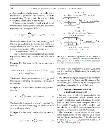
expansions, often used in mathematical model- FIGURE 2.1 Functional dependence on one variable as
ing. (A) a linear and (B) a nonlinear combination of the FB ele-
ments f i (x), i = 1,...,n.From[109], used with permission
Example 2.1. We have the Taylor series expan- from Moscow Aviation Institute.
sion, i.e.,
n
The basis of this expansion is {u i (x)} ,andthe
2 i=0
F(x) = a 0 + a 1 (x − x 0 ) + a 2 (x − x 0 ) + ···
(2.3) rule for combining FB elements is a weighted
n
+ a n (x − x 0 ) + ··· . summation.
i ∞
The basis of this expansion is {(x − x 0 ) } ,and In all these examples, the generated solutions
i=0
the rule for combining FB elements is a weighted are represented by linear combinations of ba-
summation. sis elements, parametrized by the corresponding
weights associated with each FB element.
Example 2.2. We have the Fourier series expan-
sion, i.e., 2.1.1.2 Network Representation of
Functional Expansions
∞
We can give a network interpretation for
F(x) = (a i cos(ix) + b i sin(ix)). (2.4)
functional expansions, which allows us to
i=0
identify similarities and differences between
their variants. Such description provides a fur-
∞
The basis of this expansion is {cos(ix),sin(ix)} ,
i=0
and the rule for combining FB elements is a ther simple transition to ANN models and
also allows to establish interrelations between
weighted summation.
traditional-type models and ANN models.
Example 2.3. We have the Galerkin expansion, The structural representation of the func-
i.e., tional dependence on one variable as a linear
and nonlinear combination of the elements of
n

y(x) = u 0 (x) + c i u i (x). (2.5) the basis f i (x), i = 1,...,n, is shown in Fig. 2.1A
and Fig. 2.1B, respectively.
i=1