Page 49 - Neural Network Modeling and Identification of Dynamical Systems

2.1 ARTIFICIAL NEURAL NETWORK STRUCTURES 37

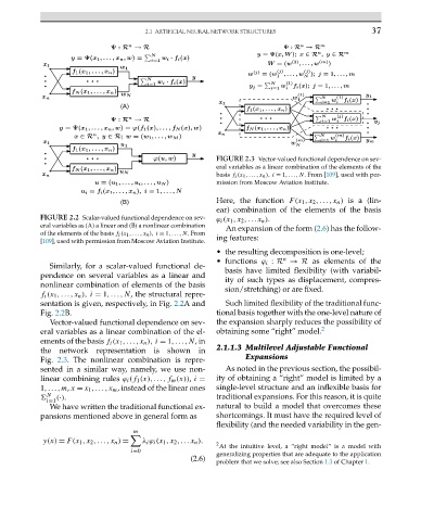
FIGURE 2.3 Vector-valued functional dependence on sev-
eral variables as a linear combination of the elements of the
basis f i (x 1 ,...,x n ), i = 1,...,N.From[109], used with per-
mission from Moscow Aviation Institute.
Here, the function F(x 1 ,x 2 ,...,x n ) is a (lin-
ear) combination of the elements of the basis
FIGURE 2.2 Scalar-valued functional dependence on sev- ϕ i (x 1 ,x 2 ,...x n ).
eral variables as (A) a linear and (B) a nonlinear combination An expansion of the form (2.6) has the follow-
of the elements of the basis f i (x 1 ,...,x n ), i = 1,...,N.From
[109], used with permission from Moscow Aviation Institute. ing features:
• the resulting decomposition is one-level;
n
• functions ϕ i : R → R as elements of the
Similarly, for a scalar-valued functional de- basis have limited flexibility (with variabil-
pendence on several variables as a linear and ity of such types as displacement, compres-
nonlinear combination of elements of the basis sion/stretching) or are fixed.
f i (x 1 ,...,x n ), i = 1,...,N, the structural repre-
sentation is given, respectively, in Fig. 2.2Aand Such limited flexibility of the traditional func-
Fig. 2.2B. tional basis together with the one-level nature of
Vector-valued functional dependence on sev- the expansion sharply reduces the possibility of
eral variables as a linear combination of the el- obtaining some “right” model. 2
ements of the basis f i (x 1 ,...,x n ), i = 1,...,N,in
2.1.1.3 Multilevel Adjustable Functional
the network representation is shown in
Expansions
Fig. 2.3. The nonlinear combination is repre-
sented in a similar way, namely, we use non- As noted in the previous section, the possibil-
linear combining rules ϕ i (f 1 (x),...,f m (x)), i = ity of obtaining a “right” model is limited by a
1,...,m, x = x 1 ,...,x m , instead of the linear ones single-level structure and an inflexible basis for
N (·). traditional expansions. For this reason, it is quite
i=1
We have written the traditional functional ex- natural to build a model that overcomes these
pansions mentioned above in general form as shortcomings. It must have the required level of
flexibility (and the needed variability in the gen-
m

y(x) = F(x 1 ,x 2 ,...,x n ) = λ i ϕ i (x 1 ,x 2 ,...x n ).
2 At the intuitive level, a “right model” is a model with
i=0 generalizing properties that are adequate to the application
(2.6)
problem that we solve; see also Section 1.3 of Chapter 1.