Page 50 - Neural Network Modeling and Identification of Dynamical Systems

38 2. DYNAMIC NEURAL NETWORKS: STRUCTURES AND TRAINING METHODS

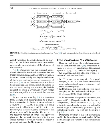
FIGURE 2.4 Multilevel adjustable functional expansion. From [109], used with permission from Moscow Aviation Insti-
tute.
erated variants of the required model), by form- 2.1.1.4 Functional and Neural Networks
ing it as a multilevel network structure and by Thus, we can interpret the model as an expan-
appropriate parametrization of the elements of sion on the functional basis (2.6), where each el-
this structure. ement ϕ i (x 1 ,x 2 ,...x n ) transforms n-dimensional
Fig. 2.4 shows how we can construct a mul- input x = (x 1 ,x 2 ,...x n ) in the scalar output y.
tilevel adjustable functional expansion. We see We can distinguish the following types of el-
that in this case, the adjustment of the expansion ements of the functional basis:
is carried out not only by varying the coefficients
of the linear combination, as in expansions of • the FB element as an integrated (one-stage)
n
the type (2.6). Now the elements of the func- mapping ϕ i : R → R that directly transforms
tional basis are also parametrized. Therefore, in some n-dimensional input x = (x 1 ,x 2 ,...x n )
the process of solving the problem, the basis is to the scalar output y;
adjusted to obtain a dynamical system model • the FB element as a compositional (two-stage)
which is acceptable in the sense of the criterion mapping of the n-dimensional input x =
(1.30). (x 1 ,x 2 ,...x n ) to the scalar output y.
As we can see from Fig. 2.4, the transition In the two-stage (compositional) version, the
from a single-level decomposition to a multi- mapping R → R is performed in the first stage,
n
level one consists in the fact that each element “compressing” the vector input x = (x 1 ,x 2 ,...x n )
ϕ
ϕ j (v,w ), j = 1,...,M, is decomposed using to the intermediate scalar output v,which in the
ψ
some functional basis {ψ k (x,w )},j = 1,...,K. second stage is additionally processed by the
Similarly, we can construct the expansion of the output mapping R → R to obtain the output y
ψ
elements ψ k (x,w ) for another FB, and so on, (Fig. 2.5).
the required number of times. This approach Depending on which of these FB elements are
gives us the network structure with the re- used in the formation of network models (NMs),
quired number of levels, as well as the required the following basic variants of these models are
parametrization of the FB elements. obtained: