Page 107 - Numerical Analysis Using MATLAB and Excel

Chapter 3 Sinusoids and Phasors

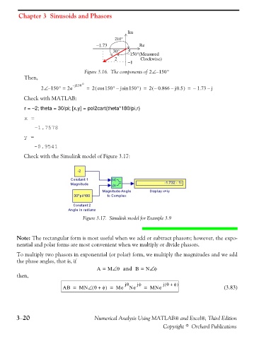
Im
210°
−1.73 Re
30°
−150°(Measured
2 Clockwise)
−1

∠
Figure 3.16. The components of 2 – 150°
Then,
j – 150°
(
)
)
(
∠
2 – 150° = 2e = 2 cos 150° – jsin 150° = 2 – 0.866 – j0.5 = – 1.73 – j
Check with MATLAB:
r = −2; theta = 30/pi; [x,y] = pol2cart(theta*180/pi,r)
x =

-1.7578
y =

-0.9541
Check with the Simulink model of Figure 3.17:

Figure 3.17. Simulink model for Example 3.9

Note: The rectangular form is most useful when we add or subtract phasors; however, the expo-
nential and polar forms are most convenient when we multiply or divide phasors.

To multiply two phasors in exponential (or polar) form, we multiply the magnitudes and we add
the phase angles, that is, if
∠
∠
A = M θ and B = N φ
then,
jθ jφ j θ ( φ + )
AB = MN ( θ∠ φ + ) = Me Ne = MNe (3.83)

3−20 Numerical Analysis Using MATLAB® and Excel®, Third Edition
Copyright © Orchard Publications