Page 146 - Numerical Analysis Using MATLAB and Excel

Chapter 4 Matrices and Determinants

I 1 219 135 81 100 219 22.46
1
---------
I = I = --------- 135 150 90 0 = 100 135 = 13.85
2 975 975
I 3 81 90 119 0 81 8.31
Check with MATLAB:

R=[10 −9 0; −9 20 −9; 0 −9 15]; V=[100 0 0]'; I=R\V

I =
22.4615
13.8462
8.3077
We can also use subscripts to address the individual elements of the matrix. Accordingly, the
above script could also have been written as:

R(1,1)=10; R(1,2)=−9; % No need to make entry for A(1,3) since it is zero.
R(2,1)=−9; R(2,2)=20; R(2,3)=−9; R(3,2)=−9; R(3,3)=15; V=[100 0 0]'; I=R\V

I =
22.4615
13.8462
8.3077
Spreadsheets also have the capability of solving simultaneous equations using the inverse matrix
method. For instance, we can use Microsoft Excel’s MINVERSE (Matrix Inversion) and MMULT
(Matrix Multiplication) functions, to obtain the values of the three currents in Example 4.17.

The procedure is as follows:

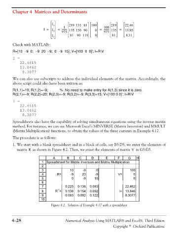
1. We start with a blank spreadsheet and in a block of cells, say B3:D5, we enter the elements of
matrix as shown in Figure 4.2. Then, we enter the elements of matrix in G3:G5.
V
R
A B C D E F G H
1 Spreadsheet for Matrix Inversion and Matrix Multiplication
2
3 10 -9 0 100
4 R= -9 20 -9 V= 0
5 0 -9 15 0
6
7 0.225 0.138 0.083 22.462
-1
8 R = 0.138 0.154 0.092 I= 13.846
9 0.083 0.092 0.122 8.3077
10
Figure 4.2. Solution of Example 4.17 with a spreadsheet

4−28 Numerical Analysis Using MATLAB® and Excel®, Third Edition

Copyright © Orchard Publications