Page 148 - Numerical Analysis Using MATLAB and Excel

Chapter 4 Matrices and Determinants

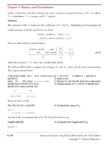
terms, collecting, and then writing the above relations in matrix form as YV = I , where
Y = admittan ce , V = voltage , and I = current .
Solution:

Y
The elements of the matrix are the coefficients of V 1 and V 2 . Simplifying and rearranging the
nodal equations of (4.60) and (4.61), we obtain

)
( 0.0218 – j0.005 V – 0.01V = 2
1
2
)
– 0.01V + ( 0.03 + j0.01 V = j1.7
1
2
Next, we write (4.62) in matrix form as
0.0218 – j0.005 – 0.01 V 1 2
– 0.01 0.03 + j0.01 V 2 = j1.7 (4.62)
⎧ ⎪ ⎪ ⎪ ⎪ ⎪ ⎨ ⎪ ⎪ ⎪ ⎪ ⎪ ⎩ ⎧ ⎨ ⎩ ⎧ ⎨ ⎩
Y V I

where the matrices , , and are as indicatedin (4.63).
YV
I
We will use MATLAB to compute the voltages V 1 and V 2 , and to do all other computations.
The script is shown below.

Y=[0.0218−0.005j −0.01; −0.01 0.03+0.01j]; I=[2; 1.7j]; V=Y\I; % Define Y, I, and find V
fprintf('\n'); % Insert a line
disp(' V1 V2'); disp(' ------------------'); % Display V1 and V2 with dash line underneath
fprintf('%9.3f %9.3f\n',V(1),V(2)) % Display values of V1 and V2 in tabular form
fprintf('\n')% Insert another line
V1 V2
------------------
104.905 53.416
Next, we find I X from

R3=100; IX=(V(1)−V(2))/R3 % Compute the value of I
X
IX =
0.5149 - 0.0590i
and this is the rectangular form of I X . For the polar form we use

magIX=abs(IX) % Compute the magnitude of I
X
magIX =

4−30 Numerical Analysis Using MATLAB® and Excel®, Third Edition

Copyright © Orchard Publications