Page 173 - Numerical Analysis Using MATLAB and Excel

Chapter 5 Differential Equations, State Variables, and State Equations

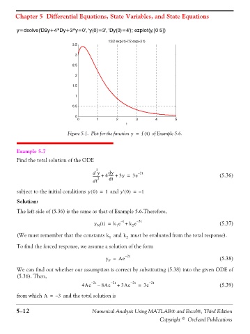
y=dsolve('D2y+4*Dy+3*y=0', 'y(0)=3', 'Dy(0)=4'); ezplot(y,[0 5])

13/2 exp(-t)-7/2 exp(-3 t)
3.5

3
2.5

2

1.5

1
0.5

0
0 1 2 3 4 5
t
Figure 5.1. Plot for the function y = f t() of Example 5.6.

Example 5.7

Find the total solution of the ODE

2
dy
d y + 4------ + 3y = 3e – 2t (5.36)
t d 2 dt
subject to the initial conditions y0() = 1 and y' 0() = – 1

Solution:
The left side of (5.36) is the same as that of Example 5.6.Therefore,

t –
y () = k e + k e – 3t (5.37)
t
N
2
1
(We must remember that the constants k 1 and k 2 must be evaluated from the total response).
To find the forced response, we assume a solution of the form
y = Ae – 2t (5.38)
F
We can find out whether our assumption is correct by substituting (5.38) into the given ODE of
(5.36). Then,
4Ae – 2t – 8Ae – 2t + 3Ae – 2t = 3e – 2t (5.39)

from which A = – 3 and the total solution is

5−12 Numerical Analysis Using MATLAB® and Excel®, Third Edition

Copyright © Orchard Publications