Page 176 - Numerical Analysis Using MATLAB and Excel

Using the Method of Undetermined Coefficients for the Forced Response

y =
-exp(-3*t)-2*exp(-3*t)*t
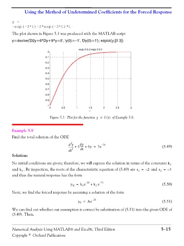
The plot shown in Figure 5.3 was produced with the MATLAB script

y=dsolve('D2y+6*Dy+9*y=0', 'y(0)=−1', 'Dy(0)=1'); ezplot(y,[0 3])

-exp(-3 t)-2 exp(-3 t) t
0
-0.1
-0.2
-0.3
-0.4
-0.5
-0.6
-0.7
-0.8
-0.9
-1
0 0.5 1 1.5 2 2.5 3
t
Figure 5.3. Plot for the function y = f t() of Example 5.8.

Example 5.9

Find the total solution of the ODE
2
dy
d y + 5------ + 6y = 3e – 2t (5.49)
t d 2 dt
Solution:

No initial conditions are given; therefore, we will express the solution in terms of the constants k 1

and k 2 . By inspection, the roots of the characteristic equation of (5.49) are s = – 2 and s = – 3
2
1
and thus the natural response has the form
y N = k e – 2t + k e – 3t (5.50)
1
2
Next, we find the forced response by assuming a solution of the form

y = Ae – 2t (5.51)
F
We can find out whether our assumption is correct by substitution of (5.51) into the given ODE of
(5.49). Then,

Numerical Analysis Using MATLAB® and Excel®, Third Edition 5−15

Copyright © Orchard Publications