Page 175 - Numerical Analysis Using MATLAB and Excel

Chapter 5 Differential Equations, State Variables, and State Equations

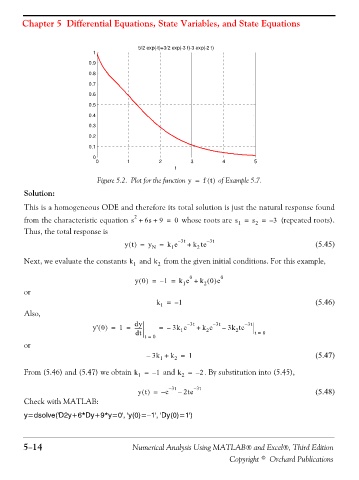
5/2 exp(-t)+3/2 exp(-3 t)-3 exp(-2 t)
1
0.9
0.8
0.7
0.6
0.5
0.4
0.3
0.2
0.1
0
0 1 2 3 4 5
t
Figure 5.2. Plot for the function y = f t() of Example 5.7.
Solution:
This is a homogeneous ODE and therefore its total solution is just the natural response found

2
from the characteristic equation s + 6s + 9 = 0 whose roots are s = s = – 3 (repeated roots).
2
1
Thus, the total response is
yt() = y N = k e – 3t + k te – 3t (5.45)
1
2
Next, we evaluate the constants k 1 and k 2 from the given initial conditions. For this example,

0
y0() = – 1 = k e + k 0()e 0
2
1
or
k = – 1 (5.46)
1
Also,
dy – 3t – 3t – 3t
y' 0() = 1 = ------ = – 3k e + k e – 3k te
dt 1 2 2 t = 0
t = 0
or
– 3k + k = 1 (5.47)
1
2
From (5.46) and (5.47) we obtain k = – 1 and k = – 2 . By substitution into (5.45),
1
2
yt() = e – – 3t – 2te – 3t (5.48)
Check with MATLAB:

y=dsolve('D2y+6*Dy+9*y=0', 'y(0)=−1', 'Dy(0)=1')

5−14 Numerical Analysis Using MATLAB® and Excel®, Third Edition

Copyright © Orchard Publications