Page 179 - Numerical Analysis Using MATLAB and Excel

Chapter 5 Differential Equations, State Variables, and State Equations

ODE with constant coefficients.

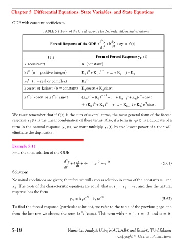
TABLE 5.1 Form of the forced response for 2nd order differential equations

2
d y dy
Forced Response of the ODE a-------- + b------ + cy = ft()
dt 2 dt

t
ft() Form of Forced Response y ()
F
k (constant) K (constant)

n
n
kt n ( = positive integer) K t + K t n – 1 + … + K n – 1 t + K n
0
1
rt rt
r
ke ( =real or complex) Ke
α
kcos αt or ksin αt ( =constant) K cosαt + K sin αt
2
1
n
n rt
n rt
rt
kt e cos αt or k t e sin αt ( K t + K t n – 1 + … + K n – 1 t + K ) n e cos αt
1
0
rt
n
(
+ K t + K t n – 1 + … + K n – 1 t + K ) n e sin αt
0
1
We must remember that if ft() is the sum of several terms, the most general form of the forced
response y t() is the linear combination of these terms. Also, if a term in y t() is a duplicate of a
F
F
term in the natural response y () , we must multiply y t() by the lowest power of that will
t
t
N
F
eliminate the duplication.
Example 5.11
Find the total solution of the ODE
2
dy
d y + 4------ + 4y = te – 2t – e – 2t (5.61)
t d 2 dt
Solution:
No initial conditions are given; therefore we will express solution in terms of the constants k 1 and
k 2 . The roots of the characteristic equation are equal, that is, s = s = – 2 , and thus the natural
1
2
response has the form
– 2t – 2t
y N = k e + k te (5.62)
1
2
To find the forced response (particular solution), we refer to the table of the previous page and
n rt
from the last row we choose the term kt e cos αt . This term with n = , 1 r = – , 2 and α = , 0

5−18 Numerical Analysis Using MATLAB® and Excel®, Third Edition

Copyright © Orchard Publications