Page 281 - Numerical Analysis Using MATLAB and Excel

Divided Differences

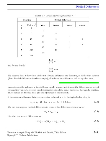
TABLE 7.3 Divided differences for Example 7.1
Function Divided Differences

x fx() = x 3 First Second Third Fourth
0 0
1
1 1 4
13 1
3 27 8 0
37 1
4 64 14 0
93 1
7 343 20
193
9 729

4 – 8
------------ = 1
0 – 4
and for the fourth

1 – 1 0
------------ =
0 – 4
We observe that, if the values of the nth divided difference are the same, as in the fifth column
(third divided differences for this example), all subsequent differences will be equal to zero.

In most cases, the values of in a table are equally spaced. In this case, the differences are sets of
x
consecutive values. Moreover, the denominators are all the same; therefore, they can be omitted.
These values are referred to as just the differences of the function.

If the constant difference between successive values of is , the typical value of x k is
x
h
,,,
,
,
x = x + kh for k = … 2 – 1012 … (7.3)
–
,
0
k
We can now express the first differences in terms of the difference operator as
Δ
Δf = f k + 1 – f k (7.4)
k
Likewise, the second differences are
2
Δ f = ΔΔf ) ( k Δ = f k + 1 – Δf k (7.5)
k

Numerical Analysis Using MATLAB® and Excel®, Third Edition 7−3
Copyright © Orchard Publications