Page 283 - Numerical Analysis Using MATLAB and Excel

Divided Differences

Solution:

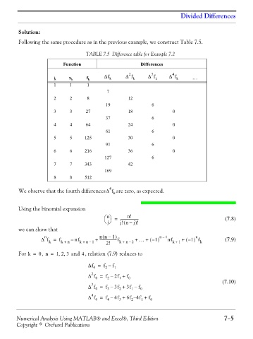
Following the same procedure as in the previous example, we construct Table 7.5.

TABLE 7.5 Difference table for Example 7.2

Function Differences

4
3
2
k x k f k Δf k Δ f k Δ f k Δ f k …
1 1 1
7
2 2 8 12
19 6
3 3 27 18 0
37 6
4 4 64 24 0
61 6
5 5 125 30 0
91 6
6 6 216 36 0
127 6
7 7 343 42
169
8 8 512

4
We observe that the fourth differencesΔ f k are zero, as expected.

Using the binomial expansion
n!
n
⎛⎞ = --------------------- (7.8)
j ⎝⎠ j! n – !
)
(
j
we can show that
(
n
n
)
Δ f = f k + n – nf k + n – 1 + nn – 1 ) k + n – 2 + … + – ( 1 ) n – 1 nf k + 1 – ( + 1 f k (7.9)
--------------------f
k
2!
,,
For k = 0 , n = 1 2 3 and , relation (7.9) reduces to
4
Δf = f – f 1
0
2
2
Δ f = f – 2f + f 0
1
2
0
3
Δ f = f – 3f + 3f – f 0 (7.10)
1
3
0
2
4
Δ f = f – 4f + 6f – 4f + f 0
1
4
0
2
3
Numerical Analysis Using MATLAB® and Excel®, Third Edition 7−5
Copyright © Orchard Publications